The upskilling trap is the most counterintuitive finding in the financial independence framework, not because the math is complex, but because it contradicts a story that feels true and is, in most other contexts, correct.
The story: skill up, earn more, accumulate faster, reach freedom sooner. This chain of causation is so intuitive that it shapes an enormous fraction of engineering career decisions. Engineers sacrifice evenings and weekends to study for promotions, negotiate aggressively for above-market compensation, and strategically target high-compensation firms. The implicit model is that more income = earlier freedom.
The formula disagrees. And the disagreement is not a rounding error.
The Mechanism, Step by Step
Return to the time-to-financial-independence formula, which derives from the financial independence condition and the accumulation equation:
t = ln([r(1 − SR)] / [WR × SR] + 1) / ln(1 + r)Where SR = savings rate, r = real investment return, WR = withdrawal rate. Income does not appear. The timeline is governed entirely by savings rate.
This result has a specific implication for raises: a raise that does not change the savings rate does not change the timeline. Full stop.
More precisely: if income increases by 30% and expenses increase by 30% to match, the savings rate is unchanged (SR = (I − E)/I = (1.3I − 1.3E)/1.3I = (I − E)/I). The formula produces the same value of t. The raise was, in terms of timeline to freedom, inert.
But there is a worse case. A raise that increases spending proportionally more than it increases saving reduces the savings rate. And a lower savings rate means a longer timeline. The engineer who receives a raise and allows lifestyle creep to absorb most of it has not just gained nothing. They have moved backward.
The Three Raise Scenarios
Three engineers each earn $150,000/year and save 30% ($45,000/year, $105,000 in expenses). Each receives a $50,000 raise to $200,000/year. What happens to their time-to-FI?
Scenario A: No savings rate adjustment (lifestyle absorbs the raise): Engineer A increases spending to $155,000/year and saves only $45,000/year (unchanged in absolute dollars). New savings rate: $45,000 / $200,000 = 22.5% New years-to-FI at 7% return, 4% WR: approximately 33 years Original years-to-FI at 30%: approximately 27 years Result: +6 years on the timeline despite the raise.
Scenario B: Maintain savings rate (proportional increase): Engineer B keeps savings rate at 30%, saving $60,000/year, spending $140,000/year. Years-to-FI at 30%: approximately 27 years Result: no change to timeline.
Scenario C: Increase savings rate (direct the surplus): Engineer C maintains $105,000 in spending (same lifestyle) and saves $95,000/year. New savings rate: $95,000 / $200,000 = 47.5% New years-to-FI: approximately 16 years Result: −11 years off the timeline from the same raise.
The difference between Scenario A and Scenario C is 17 years of mandatory employment. Both engineers received identical raises. One bought 11 years of freedom. The other spent 6 years of freedom before they earned them. The chart below plots all three freedom dates from the same starting point.
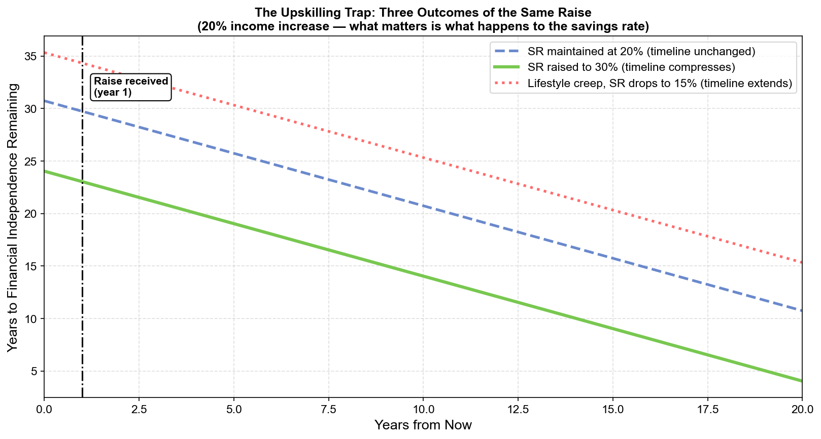
The divergence is immediate: three identical raises producing three dramatically different freedom dates. The raise is not the variable. The savings rate response is the variable.
Why This Happens: The Moving Goalposts Problem
The Scenario A outcome has a second mechanism that the formula captures but deserves explicit attention: lifestyle creep does not just reduce the savings rate. It also moves the FI target in the wrong direction.
The FI target is 25× annual expenses. If annual expenses increase from $105,000 to $155,000, the target increases from $2,625,000 to $3,875,000, an increase of $1,250,000 in required portfolio value. At the same time, annual contributions remained flat at $45,000.
The engineer just:
- Reduced the contribution rate to the portfolio (SR dropped from 30% to 22.5%)
- Increased the target portfolio size by $1,250,000
Both changes work against the timeline simultaneously. The goalposts moved further away at exactly the moment the velocity toward them decreased. This is the double penalty of the upskilling trap.
The mechanism is easy to miss because each individual spending decision looks reasonable. A nicer apartment in a better neighborhood, a better car because the commute is now 45 minutes each way, a gym membership because the new peers all have them, a better dining budget because the new salary level changes expectations. None of these feels like a financial strategy error. Each is individually defensible. But the aggregate is a systematic rewriting of the FI target.
The Correct Protocol for a Raise
The upskilling trap is avoidable with a specific protocol, applied mechanically at every income increase:
Step 1: Calculate the raise’s savings potential at constant lifestyle.
If your income goes from I₀ to I₁ while expenses stay at E₀:
New SR = (I₁ − E₀) / I₁This is the maximum savings rate accessible from the raise without any lifestyle adjustment. It is the efficiency ceiling. If the raise is substantial and lifestyle is held constant, this number can be dramatically higher than the pre-raise savings rate.
Step 2: Decide the lifestyle allocation.
You are entitled to spend some portion of the raise on genuine quality of life improvements, the ones that pass the hedonic adaptation test (low-adaptation, high-value) and the Freedom Cost Matrix (reasonable years-of-work price). The question is not “should I spend any?” but “how much, on what, with what freedom cost?”
A reasonable rule: allocate no more than 30–40% of the after-tax raise increment to lifestyle improvements. The remaining 60–70% goes directly to savings rate increase.
At a $50,000 gross raise (approximately $30,000 after-tax at high income brackets), 60–70% directed to savings means $18,000–$21,000 of additional annual savings. Spending $9,000–$12,000 of the after-tax increment on lifestyle improvements.
Step 3: Automate before the lifestyle inflates.
The adaptation process that drives the upskilling trap is not instantaneous. After a raise, the brain takes time to recalibrate what “normal” spending feels like. The window between the first paycheck at the new rate and full lifestyle adaptation is the capture window.
Increase automated contributions immediately, before the first paycheck at the new rate, if possible. Direct the savings rate increase to the investment automation pipeline before the discretionary budget has a chance to absorb the new inflow. You cannot spend what has never appeared in your checking account.
The Upskilling Paradox Resolved
The upskilling trap does not argue that earning more is counterproductive. It argues that earning more without a savings rate adjustment is counterproductive. These are different claims.
The correct framing is that upskilling has two outputs:
- Increased income (the part that is visible and celebrated)
- Increased freedom, but only if the savings rate increases along with income
The second output is not automatic. It requires an explicit decision to capture the raise as savings rate improvement instead of as lifestyle improvement. Without that decision, the first output (income increase) is captured entirely by the second behavioral mechanism (hedonic adaptation and spending inflation), and the net effect on the freedom timeline is zero or negative.
Engineers are systematically trained to optimize for the first output. The industry rewards it, the culture celebrates it, and the career framework is entirely structured around it. The second output requires an override: a deliberate redirection of the raise before the adaptation process runs.
The upskilling itself is correct. The raise is worth pursuing. The trap is in the assumption that pursuing the raise is sufficient. The raise is the throughput. The savings rate is the accumulation. Throughput without accumulation is the vanity metric problem applied to raises. The same decoupling that separates income from wealth, in aggregate, operates at the level of each individual raise.
The Compounding Consequence
The raises that fail to increase the savings rate do not just miss an opportunity. They set a compounding baseline.
Lifestyle that adapts upward at year 1 creates expectations for year 2. The year 2 raise is now evaluated against the year 1 lifestyle as baseline. If year 2 lifestyle also expands with the raise, year 3 starts at an even higher floor. After five years of raises absorbed by lifestyle, the engineer has a high income, a high-cost lifestyle, high fixed obligations, and exactly the savings rate they started with. Possibly lower.
The compound effect runs in the right direction when savings rates increase with each raise. After five years of raises where 70% of each after-tax increment went to savings, the engineer has a dramatically higher savings rate, a growing portfolio, and modest lifestyle expansion. The Freedom Velocity Curve position has moved substantially left. The timeline has compressed.
The difference between these two five-year outcomes is not willpower or sacrifice. It is a single decision applied consistently: direct the majority of each raise to savings rate improvement before the adaptation process can absorb it. The rest of the system (the compounding, the timeline compression, the growing optionality) follows automatically from that one protocol.
The upskilling trap closes the moment you decide that the raise is a financial rate-of-freedom improvement, not a lifestyle upgrade event.
This article is adapted from Chapter 3 of Debugging Your Personal Finance, which presents the upskilling trap as the final behavioral algorithm running against the financial independence timeline, alongside Parkinson’s Second Law, the Diderot Effect, and the Hedonic Treadmill. Together, these four mechanisms explain why income growth so frequently fails to produce equivalent timeline compression, and why the savings rate, not the income level, is the primary controllable variable in the freedom formula.