Two investors earn the same 30 yearly returns in a different order. One ends with 13.6 million dollars. The other runs out of money. Only the sequence changed.
That sentence should feel impossible, because for most of your investing life it is. If you buy a lump sum and never touch it again, the order of your returns is genuinely irrelevant. Multiplication commutes, so shuffling the years cannot change where you land. The surprise is that the instant you add money or draw money out, that harmless-looking property breaks, and it breaks hard. This is sequence of returns risk, and it is one of the few places in personal finance where a fact from arithmetic flips into a fact about whether you eat.
I will show it with a real backtest. I took a fixed set of 30 actual annual S&P total returns from Robert J. Shiller’s monthly dataset (econ.yale.edu/~shiller), the calendar years 1994 through 2023, dividends reinvested. Then I applied that identical set of numbers in two different orders and watched what happened to a lump sum, a saver, and a retiree.
A system with feedback behaves differently from one without
Start with the engineering frame, because it makes the whole thing obvious in hindsight.
A buy-and-hold lump sum is an open-loop system. You put in a signal at the start, the market applies a chain of multiplications, and you read the output at the end. There is no path from the output back into the input. Your balance in year 20 does not change how much money is riding through year 21, because the amount riding is always just whatever the market left you, untouched. In a pure chain of multiplications the operations commute, so the sequence of the multipliers is invisible in the final product.
Now attach a cash flow. A saver adds a fixed deposit every year. A retiree removes a fixed withdrawal every year. Either way you have created a feedback path. The size of this year’s contribution or withdrawal is fixed in dollars, but its weight relative to the portfolio depends on how big the portfolio already is, and how big the portfolio already is depends on every return that came before. The output now feeds back into the state that the next return acts on. That is the definition of a closed-loop system, and closed-loop systems care deeply about order, because the same disturbance hitting early lands on a different state than it does hitting late.
So the thesis is a claim about system structure. With no feedback, order is irrelevant. Add feedback through cash flows, and order becomes one of the largest variables you have. The rest of this article is the numbers that prove it.
The lump sum lands in the same place no matter what
Here is the control case. Invest 100,000 dollars once, add nothing, withdraw nothing, and let the 30 returns run.
I applied the returns in two deliberately extreme orders. “Good years early” sorts all 30 returns from best to worst, so the huge gains of the late 1990s bull come first and the 39 percent crash of 2008 comes near the end. “Good years late” is the exact reverse, worst to best, so the account eats the 2008-sized loss up front and the 38 percent gains arrive last. These are the same 30 numbers, just reversed.
The good-years-early lump sum ends at 1,757,224 dollars. The good-years-late lump sum ends at 1,757,224 dollars. They match to the cent. The growth factor is 17.57 times the starting capital either way, because 100,000 dollars multiplied by 30 growth factors gives the same product no matter which factor you write first. The arithmetic mean of the 30 annual returns is 11.56 percent, and for a lump sum that average, compounded over the fixed set of years, is the entire story. Order contributes nothing.
This is the property people quietly assume holds everywhere. It does not. It holds here precisely because nothing touches the account between the start and the end.
For a saver, good years late beat good years early by ten to one
Now give the account a cash flow. The saver starts from zero and invests 10,000 dollars at the beginning of every year for 30 years, then lets that year’s return act on the balance. Same 30 returns, same two orders.
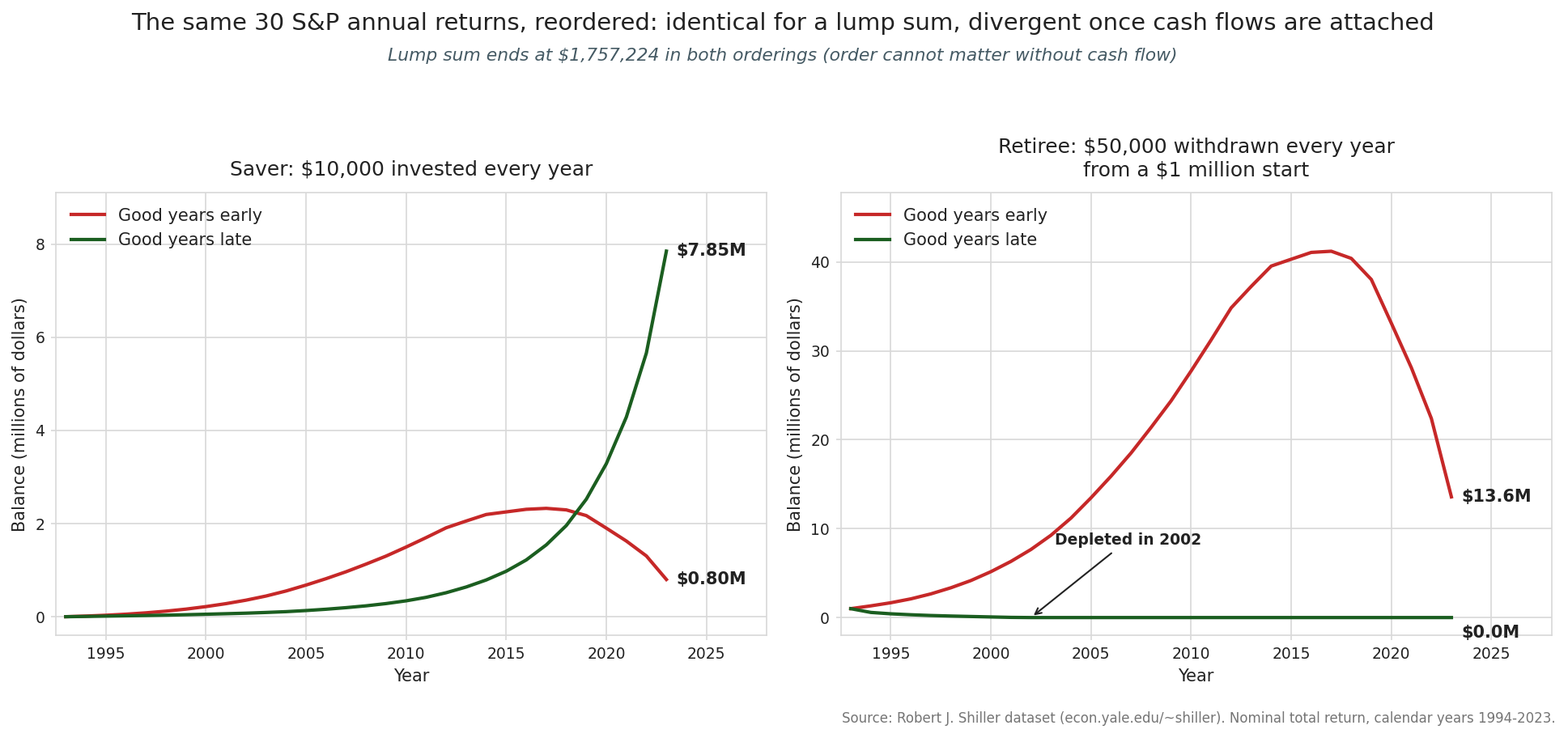
Good years early ends at 799,025 dollars. Good years late ends at 7,850,908 dollars. The saver who happened to receive the strong years at the end finished with almost ten times as much money, a factor of 9.8, off an identical string of returns and identical 10,000 dollar deposits. The gap between the two outcomes is 7.05 million dollars, created by sequence alone.
The reason is a mismatch between where your money is and when the returns show up. Early in a savings plan the balance is tiny, because you have only made a few deposits. A 38 percent gain on a 20,000 dollar balance is worth about 7,600 dollars. Late in the plan the balance is enormous, because 30 years of deposits and compounding have piled up. That same 38 percent gain on a 6 million dollar balance is worth 2.3 million. Good returns are only as valuable as the balance they land on, and a saver’s balance is smallest at the start and largest at the end. Putting the best years last aims the biggest multipliers at the biggest balance. Putting them first wastes them on a nearly empty account, and then hands the crash to the account after it has grown large.
The left panel of the figure shows both saver paths on the same axes. The good-years-late line is nearly flat for years, then bends sharply upward as the late gains compound on top of decades of deposits. The good-years-early line climbs early, then stalls and drifts downward as the reordered losses chew through a balance that has nothing left coming to rescue it. The two curves start from the same zero, receive the same money, and end more than 7 million dollars apart.
If you are still accumulating, this is mostly good news dressed as a warning. A bad decade early in your saving life, when your balance is small, does limited damage, and a strong decade near the end, when your balance is large, does most of the work. The uncomfortable version of the same fact is that the returns in the five to ten years right before you stop working carry far more weight than the returns in your first decade, because they act on your largest balance.
For a retiree, the order decides whether the money survives at all
The withdrawal case is where sequence stops being a matter of how rich you end up and becomes a matter of whether you make it. The retiree starts with 1,000,000 dollars, withdraws 50,000 dollars at the beginning of each year, which is a 5 percent initial withdrawal rate, then lets that year’s return act on what remains. Same 30 returns, same two orders.
Good years early ends at 13,577,117 dollars. Good years late ends at zero. The account is fully depleted by 2002, nine years in, and the remaining 21 years of returns, including every one of those late 30-plus percent gains, act on an empty balance and do nothing. One ordering turns a million dollars into more than 13 million. The reverse ordering turns the same million into nothing, using the same returns and the same spending.
The mechanism is the mirror image of the saver’s, and it is brutal. A retiree draws a fixed dollar amount from a shrinking pool. When a large loss lands early, the portfolio falls at the same time the withdrawals keep taking their fixed 50,000 dollars. The account now has to recover from a lower base while continuing to fund spending, and shares sold during the downturn to cover that spending are gone. They are not there to participate when the recovery finally comes. Good returns arriving later find too little principal left to work on. In the good-years-late ordering the first several years combine steep losses with steady 50,000 dollar withdrawals, and the balance simply runs out before the good years ever arrive. In the good-years-early ordering the strong early gains lift the portfolio so far above the withdrawals that it can absorb the later crash and still finish with an enormous surplus.
The right panel of the figure shows this as starkly as the numbers do. The good-years-early retiree climbs almost vertically as early gains outrun the withdrawals. The good-years-late retiree slides down a short ramp and hits zero, marked on the chart at 2002, after which the line stays pinned to the floor while the unused good years pass overhead. Two retirees, identical starting portfolio, identical withdrawals, identical set of market returns, and one of them spends the last two decades broke.
This is why the same average return can support a comfortable retirement or produce ruin depending only on when the bad years fall. A 5 percent withdrawal rate against an average return of 11.56 percent sounds safe, and over a lump sum it would be trivially safe. Under withdrawals with the losses stacked at the front, it is fatal. The average told you nothing about the risk that actually mattered.
Line the three scenarios up and the pattern is clean. The lump sum, with no cash flow, is perfectly indifferent to order and ends at 1,757,224 dollars every time. The saver, adding money, prefers good years late and swings by a factor of ten. The retiree, removing money, is destroyed by good years late and swings between more than 13 million dollars and zero. The only variable moving across all three is the direction and existence of a cash flow. Add nothing and order cannot touch you. Add a feedback path and order becomes the dominant term.
For the accumulation years this reframes what a market crash means. A drop early in your saving life, when the balance is small, is close to harmless and can even help by lowering the prices of the shares you are still buying. The returns that decide your final balance are the ones near the finish line, when the balance is at its peak. For the withdrawal years it reframes what safety means. The danger is not a bad average. The danger is a bad opening sequence, a string of losses in the first few years of withdrawals, because that combination of falling prices and fixed spending can hollow out the principal before any recovery can reach it. The order of your returns matters as much as the average, and in retirement it can matter more.
Sources
- Robert J. Shiller, “Irrational Exuberance” monthly S&P Composite dataset, http://www.econ.yale.edu/~shiller/data.htm. Annual returns are the December-to-December change in the nominal total-return index (one twelfth of the annualized dividend reinvested each month at that month’s price), for the 30 calendar years 1994 through 2023. Arithmetic mean of those 30 annual returns is 11.56 percent; the lump-sum growth factor over the full set is 17.57 times.
- Ending balances computed for each scenario. Lump sum from 100,000 dollars ends at 1,757,224 dollars in both orderings. Saver contributing 10,000 dollars per year ends at 799,025 dollars (good years early) versus 7,850,908 dollars (good years late). Retiree withdrawing 50,000 dollars per year from 1,000,000 dollars ends at 13,577,117 dollars (good years early) versus zero, depleted by 2002 (good years late).