There is a formula that tells you exactly how much of your money to put at risk, it has been public since 1956, and almost nobody should use the number it produces. That sounds like a contradiction. It is closer to a warning label. The formula is correct, its assumptions are clean, and the gap between the assumptions and the world you actually invest in is wide enough to bankrupt anyone who ignores it.
The question the formula answers is the one every allocation decision hides. You have found something with a positive edge, meaning you expect to make money on average. How much do you commit? Betting too little wastes the edge. Betting too much destroys you, and it destroys you even when the edge is real and you were right about it the whole time. There is a size in between that grows your money faster than any other size, and it has a name.
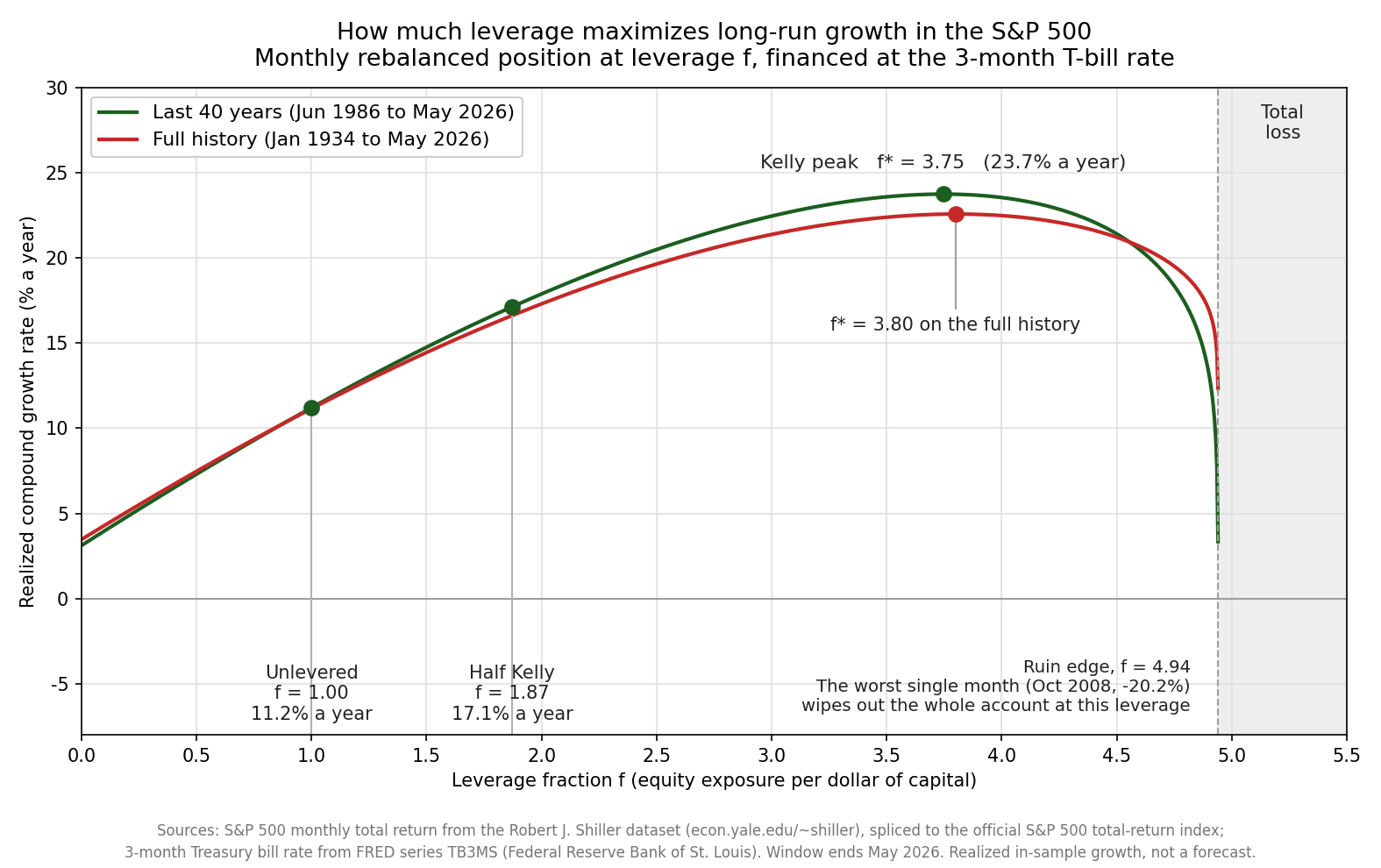
I applied that formula to real S&P 500 history instead of a coin-flip example. The dataset is the monthly S&P 500 total return series built from Robert J. Shiller’s public data (econ.yale.edu/~shiller) and spliced to the official S&P 500 total-return index, with the 3-month Treasury bill rate from FRED series TB3MS (Federal Reserve Bank of St. Louis) as the cash and borrowing rate. For each leverage fraction f, I built a portfolio that rebalances every month to hold exactly f dollars of stock per dollar of capital, borrowing the shortfall at the bill rate when f exceeds one and lending the surplus at the bill rate when f falls short of one. Then I measured what that portfolio actually compounded at over the last 40 years, June 1986 through 2026, and over the full common history back to January 1934. The chart below plots what each of those portfolios earned, realized growth rate against leverage, for both windows.
A Bell Labs Paper About Noisy Telephone Lines
The formula came out of information theory. J. L. Kelly Jr., a physicist at Bell Labs, published “A New Interpretation of Information Rate” in the Bell System Technical Journal, volume 35, number 4, July 1956, pages 917 to 926. Kelly was working on a problem that had nothing to do with markets. Claude Shannon had shown a few years earlier how much information a noisy channel can carry, and Kelly wanted a concrete interpretation of that quantity. He found one in gambling.
His setup was a gambler receiving advance results over a noisy wire. The gambler knows the tips are sometimes wrong, so the question is what fraction of the bankroll to stake on each one. Kelly showed that the fraction maximizing the long-run exponential growth rate of the bankroll is exactly the one whose growth rate equals the information rate of the channel. Information and money turned out to be the same mathematics wearing different clothes.
The mechanical insight underneath is more useful than the information-theory framing. Kelly’s gambler does not maximize expected wealth. Maximizing expected wealth tells you to bet everything on every favorable wager, which produces an enormous average outcome driven by a vanishingly rare path where you never lose, alongside near-certain ruin on every other path. Kelly maximizes the expected logarithm of wealth instead. Log wealth is the right target because wealth compounds multiplicatively, and the log turns a product of growth factors into a sum. Maximizing the average of that sum maximizes the rate at which your capital actually compounds along the path you will personally live through.
That distinction does the real work. Expected return is an average across parallel universes, weighted by outcomes most of which you will never see. Compound growth is what happens in the single universe you inhabit, and it is punished by volatility in a way that expected return is not.
The Version That Applies to a Stock Portfolio
Kelly’s original result was stated for discrete bets with known odds. The continuous version relevant to investing came from Robert C. Merton, “Lifetime Portfolio Selection under Uncertainty: The Continuous-Time Case,” Review of Economics and Statistics, volume 51, number 3, 1969, pages 247 to 257. Merton solved for the optimal share of wealth in a risky asset under a general utility function, and log utility is the special case that reproduces Kelly.
The answer is compact. If the risky asset has expected return μ, the risk-free rate is r, and the volatility is σ, the growth-optimal exposure is
f* ≈ (μ − r) / σ²
Everything you need to know about Kelly in practice is visible in that expression. The numerator is the edge, the excess return you expect over cash. The denominator is variance, which is volatility squared. Doubling the edge doubles the recommended position. Doubling the volatility cuts the recommended position to a quarter. Risk enters the formula squared while reward enters it linearly, which is why the answer collapses fast when an asset gets choppier.
The reason growth peaks and then falls is the drag term. The compound growth rate of a leveraged position is approximately r + f(μ − r) − f²σ²/2. The middle term is the edge you harvest, and it grows linearly with leverage. The last term is volatility drag, and it grows with the square of leverage. At low f the linear term wins. At high f the quadratic term wins, and it wins decisively. Somewhere in between the two rates of growth cross, and that crossing point is f*.
Plug in the numbers from the last 40 years of S&P 500 history. The annualized excess return over T-bills was 8.38 percent, and annualized volatility was 12.42 percent, giving a variance of 0.01542. The closed form returns f* = 5.44. That is five and a half times leverage, which should immediately make you suspicious, and the suspicion is correct.
What the Real Data Says, and Where the Formula Overshoots
The green curve in the figure is the measured answer, with no Gaussian assumption anywhere. It is the realized compound growth rate of the monthly rebalanced portfolio at every leverage from zero to 5.5, computed directly from the actual sequence of monthly returns.
It peaks at f* = 3.75, not 5.44. Growth at that peak was 23.74 percent a year. Half Kelly, f = 1.87, delivered 17.13 percent a year. The unlevered portfolio at f = 1 delivered 11.20 percent a year. The full history back to 1934, in red, peaks in nearly the same place, at f* = 3.80 with growth of 22.57 percent a year, which is at least reassuring about stability across two very different eras.
The gap between the closed form’s 5.44 and the measured 3.75 is the first honest lesson. The closed form assumes returns are lognormal with constant volatility. Real monthly equity returns have a fatter left tail than that, and the drag from a fat left tail is worse than the σ²/2 term predicts. The Gaussian formula therefore overstates how much leverage you can carry. It overstates it by nearly a third here.
There is a second overstatement hiding in the data itself. Shiller’s monthly price is an average of that month’s daily closes, which smooths the series and understates true monthly volatility. Measured on true month-end values of the official S&P 500 total-return index over the same window, annualized volatility was 14.61 percent instead of 12.42 percent. Feed that into the closed form and f* drops from 5.44 to 3.93. Since Kelly divides by variance, a modest measurement artifact in σ moves the recommendation substantially.
Then look at the right side of the chart, where the curve does something a smooth textbook parabola never does. Past f = 4.94 the portfolio does not merely grow slowly. It ceases to exist. October 2008 delivered a monthly total return of −20.19 percent in this series, and at 4.94 times leverage a single month like that consumes the entire account. Everything beyond that line is shaded because there is no growth rate to plot. The account is at zero and no subsequent return can revive it.
That cliff is the part the closed form cannot express, and it is the part that matters most. Kelly’s formula describes a smooth trade-off between edge and drag. Actual leverage introduces a hard boundary where one bad month ends the experiment permanently. The distance between the theoretical optimum of 5.44 and the ruin edge of 4.94 is negative. The formula, taken literally, recommends a position that the realized data would already have destroyed.
Why Practitioners Bet Half
Suppose you somehow knew f* exactly. You would still not want to bet it, because full Kelly is nearly unlivable.
At f = 3.75 on this data, annualized volatility of the levered portfolio was 46.46 percent, and the worst single month was −75.78 percent. Three quarters of the account gone in four weeks, on a strategy that is mathematically optimal and performing exactly as designed. Kelly’s criterion optimizes the growth rate and says nothing at all about the ride. A full Kelly bettor spends long stretches deep underwater. Under the idealized lognormal assumptions, a full Kelly portfolio will at some point be down 50 percent from its peak with probability approaching one.
The standard response is fractional Kelly, and the standard fraction is one half. It works because of an asymmetry in the shape of the curve. Near its peak the growth curve is flat, so giving up leverage costs surprisingly little growth. Betting a fraction c of Kelly captures (2c − c²) of the excess growth that full Kelly earns above the risk-free rate. At c = 0.5 that is 0.75, so half Kelly theoretically retains three quarters of the excess growth while carrying half the volatility. In this dataset the realized figure was 68 percent of the excess growth for half the volatility, which is close enough to make the point. You surrender about a quarter to a third of your growth advantage and cut your risk in half.
That trade-off has been studied formally. L. C. MacLean, W. T. Ziemba and G. Blazenko, “Growth versus Security in Dynamic Investment Analysis,” Management Science, volume 38, number 11, 1992, mapped the growth-versus-safety frontier for fractional Kelly and found the same asymmetry. Edward O. Thorp, who first applied Kelly to blackjack and then to markets, has written repeatedly that he ran fractional Kelly in practice for exactly this reason; his survey “The Kelly Criterion in Blackjack, Sports Betting, and the Stock Market” lays out both the theory and his own retreat from the full bet.
Not everyone accepted the framework. Paul A. Samuelson objected in “Why we should not make mean log of wealth big though years to act are long,” Journal of Banking & Finance, volume 3, number 4, 1979, pages 305 to 307, a paper written almost entirely in one-syllable words to make the rebuttal impossible to hide behind jargon. His argument was that maximizing log wealth is one particular utility function among many, and there is no reason a given investor’s risk preferences should match it. He was right about that. Kelly tells you how to grow fastest. Whether growing fastest is what you want is a separate question, and for most people with a finite horizon and a real nervous system, it is not.
The Number You Cannot Actually Measure
Everything above assumed the inputs were known. They are not, and this is the argument that should decide the matter.
Volatility is estimable. Sample it more finely and the estimate tightens quickly. Expected return behaves differently. Robert C. Merton showed in “On Estimating the Expected Return on the Market,” Journal of Financial Economics, volume 8, number 4, 1980, that the precision of an estimated mean return depends on the calendar length of the sample and not on how often you sample within it. Forty years of data gives you forty years of information about μ no matter how many observations you slice it into.
The consequence is stark. With volatility of 12.42 percent and 40 years of history, the standard error of the estimated excess return is 1.96 percentage points. The measured 8.38 percent therefore carries a 95 percent interval running from 4.53 percent to 12.23 percent. Push those bounds through the Kelly formula and the recommended leverage runs from 2.94 to 7.93. Forty years of data, one of the best-documented return series in existence, and the honest answer spans a factor of nearly three.
Now recall that the ruin edge sits at 4.94. A sizeable part of that confidence interval is on the far side of total loss.
The asymmetry of the error compounds the problem. Overbetting is far more costly than underbetting, because the growth curve falls away steeply on the right and flattens gently on the left. Betting half of f* costs you about a third of your excess growth. Betting twice f* takes you past the cliff. Since you cannot know f*, and since the penalty for guessing high is categorically worse than the penalty for guessing low, the rational response to uncertainty is to shade down hard. Half Kelly earns its place as the arithmetic of estimation error, and timidity has nothing to do with it.
One more caveat belongs on the record. The f* of 3.75 in the figure is an in-sample number. It is the leverage that would have been optimal for a path that has already happened, computed with perfect knowledge of that path. It is not a forecast, and nothing guarantees the next 40 years produce a similar peak. The calculation also charges borrowing at the Treasury bill rate, which no retail investor gets, and it ignores transaction costs, margin calls and taxes. Every one of those omissions pushes the real-world optimum lower than the chart shows.
Kelly gave us the correct target, which is the growth rate of capital along the path you actually travel. The formula that hits that target is exact under assumptions that reality does not honor, and it is driven by a parameter that four decades of the world’s most-studied market cannot pin down within a factor of three. The right way to hold it is as an upper bound that you deliberately stay well beneath. When the math says 3.75 and the cliff says 4.94, aiming carefully at 3.75 is the wrong instinct. Stand somewhere near one, and understand why the curve has a peak at all.