In engineering, a vanity metric is one that looks impressive on a dashboard but has zero correlation with system health. Total app downloads is the canonical example. The number goes up and to the right, it looks great on an investor slide, but if daily active users are zero the business is dead. Downloads measure throughput into the top of the funnel. They say nothing about retention, engagement, or value delivered.
In personal finance, income is the ultimate vanity metric.
Tech hubs are full of engineers wearing their salaries like badges of honor. “I just got an offer from a FAANG company at $350k total comp.” The implicit assumption is that because the throughput number is high, the system health must also be high. The data consistently shows this assumption is false.
The Decoupling Nobody Talks About
Here is the claim stated plainly: income and wealth are decoupled. A senior engineer earning $400,000 can be weeks from bankruptcy. A junior engineer earning $90,000 can be mathematically free. The link between salary and net worth is not automatic. It requires an explicit system design, and most people have never built that system.
The most extreme dataset available is professional athletes. These individuals experience super-income events, multi-year contracts worth millions, yet a National Bureau of Economic Research study found that 15.7% of NFL players file for bankruptcy within 12 years of retirement. The finding that matters most: there was no correlation between total career earnings and bankruptcy rate. Players who earned $10 million were just as likely to go broke as those who earned $2 million.
The NFL dataset is clean because the incomes are unusually high and the career windows are short, which makes the decoupling unmistakable. But the same pattern runs at every income level. A 2024 report found that 50% of US consumers earning more than $100,000 annually live paycheck to paycheck. The problem is not income. The problem is the assumption that income automatically becomes wealth.
It does not. Income is flow. Wealth is accumulation. They are different quantities, and optimizing flow does not automatically improve accumulation.
Parkinson’s Second Law: The Zero-Gap Equilibrium
The mechanism behind the decoupling is precise and predictable. In 1955, C. Northcote Parkinson stated his first law: “Work expands to fill the time available for its completion.” His second law, less famous but more financially damaging, applies directly: “Expenditures rise to meet income.”
From a systems engineering perspective, your personal finance system seeks zero-gap equilibrium. Nature abhors a vacuum. When income increases by ΔI, the system generates new perceived necessities to absorb the increment, and expenses adjust by approximately ΔE ≈ ΔI. The gap closes. Throughput increased; retention did not change.
This is not a character flaw. It is a predictable system behavior. The engineer who receives a $50,000 raise and finds themselves in the same financial position two years later has not failed through lack of discipline. They have been defeated by a system-level default behavior that was never explicitly overridden.
The override requires a deliberate architectural decision: savings rate must be increased when income increases, not maintained. This is the only intervention that decouples income from expenditure and allows throughput to become accumulation.
PAW vs. UAW: The Value Metric That Actually Measures Wealth
If income is the vanity metric, the value metric is net worth relative to age-and-income expectations. Dr. Thomas Stanley, in The Millionaire Next Door, formalized this with a diagnostic formula:
Expected Net Worth = (Age × Annual Income) / 10This formula sets a baseline: given your age and income, how much net worth should you have accumulated if you were operating at average efficiency? Individuals who significantly exceed this baseline are Prodigious Accumulators of Wealth (PAWs). Those who fall significantly below it are Under Accumulators of Wealth (UAWs).
Compare two hypothetical subjects at age 50:
Subject A (Physician, UAW)
- Annual income: $250,000
- Expected net worth: $1,250,000
- Actual net worth: $400,000
- PAW/UAW status: UAW, running at 32% of expected efficiency
Subject B (Engineer, PAW)
- Annual income: $100,000
- Expected net worth: $500,000
- Actual net worth: $1,100,000
- PAW/UAW status: PAW, running at 220% of expected efficiency
The chart below sets the two subjects side by side on both metrics.
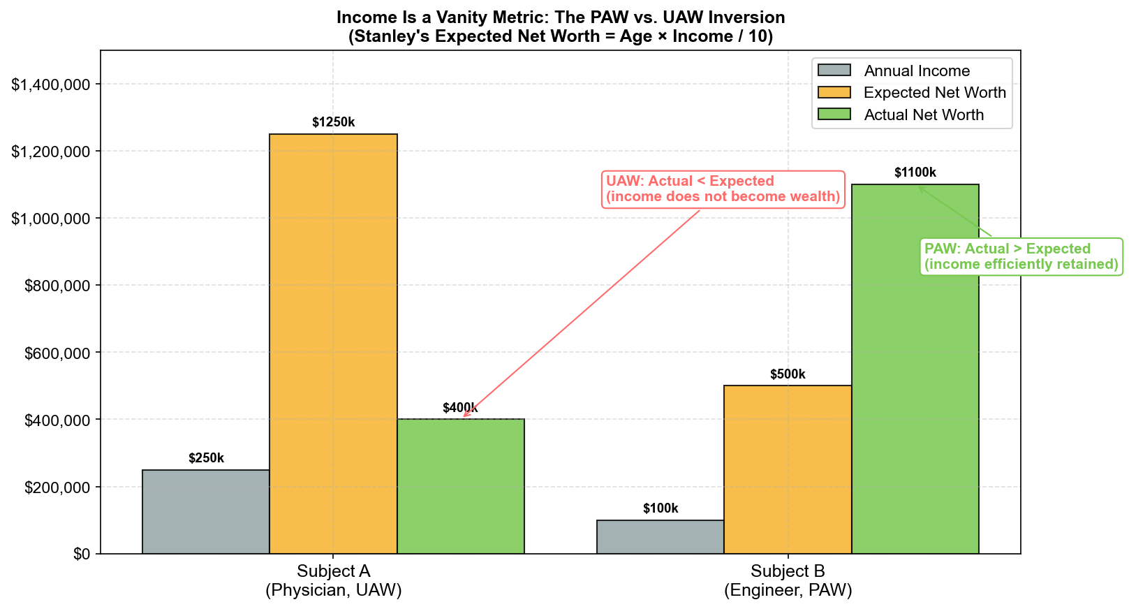
The chart makes the inversion visible. Subject A dominates the income bar, the vanity metric. Subject B dominates the actual net worth bar, the value metric. Society reads Subject A as the wealthier individual. Subject B owns their time; Subject A does not.
This is not an unusual outcome. It is the typical outcome when the system is optimized for throughput instead of retention. High income with low accumulation efficiency is exactly what Parkinson’s Second Law predicts: a high-flow, high-leak system.
The Accumulation Efficiency Score
The PAW/UAW framework has a known limitation: it assumes a linear career trajectory, which penalizes engineers who spent years in lower-paying roles before a major compensation jump. A 35-year-old who was in a PhD program until 30 and then joined a tech company at $200,000 will appear to be a UAW by the formula even if they are saving aggressively.
The more robust metric for engineers with non-linear careers is accumulation efficiency: total lifetime savings divided by total lifetime gross income. This ratio normalizes for timing and measures what actually matters: of all the income that has flowed through your system, what fraction has been retained as net worth?
A 40-year-old with $1.5M in cumulative lifetime income and $500,000 in net worth has an accumulation efficiency of 33%. A peer with $600,000 in cumulative income and $300,000 in net worth has an efficiency of 50%. The second engineer has a higher-performing financial system despite lower absolute income and lower absolute net worth.
The tracking metric is simple:
Accumulation Efficiency = Net Worth / Cumulative Lifetime Gross IncomeTarget: above 30% by age 40, above 50% by age 50. These are not arbitrary benchmarks. They are the levels at which the portfolio, compounding forward, generates enough growth to sustain a meaningful financial independence timeline.
What to Optimize Instead
The reframe from income to accumulation efficiency changes the decisions you face at every level.
At the career level: the question is not “how do I maximize my total compensation?” It is “how do I maximize the fraction of compensation that becomes net worth?” These are not the same question. A role with $300,000 total comp and a culture that produces $250,000 in annual lifestyle expansion has worse accumulation efficiency than a role with $200,000 comp and a culture that allows $100,000 in annual savings. The comp numbers are not the relevant comparison.
At the purchase level: every discretionary spending decision is an accumulation efficiency decision, not an income decision. The question “can I afford this?” is always answerable at a high income level. The question “does this purchase improve or degrade my accumulation efficiency?” is harder and more relevant.
At the measurement level: stop checking salary on Blind. Start tracking your monthly savings rate. The savings rate is the leading indicator of accumulation efficiency, the controllable input that determines the output. Income is the amplifier. Savings rate is the dial.
This article is adapted from Chapter 3 of Debugging Your Personal Finance, which derives the full proof that income cancels out of the time-to-freedom formula, introduces the Freedom Velocity Curve, and provides the framework for converting a high-throughput system into a high-accumulation one.