Not all savings rates are created equal. The relationship between how much you save and how long you must work is not linear. It is hyperbolic. Each additional percentage point of savings rate buys back a different number of years depending on where you are on the curve. The earlier you are on the curve (lower savings rates), the more years each percentage point is worth. The later you are (higher savings rates), the smaller the marginal gain.
Understanding this curve, its shape, its inflection points, and why 50% is the specific threshold that matters most, changes how engineers should think about every financial decision.
The Shape of the Curve
The Freedom Velocity Curve plots savings rate on the x-axis against years to financial independence on the y-axis. It is derived directly from the FIRE formula:
t = ln([r(1 − SR)] / [WR × SR] + 1) / ln(1 + r)At a 7% real return and 4% withdrawal rate, the curve looks like this:
| Savings Rate | Years to FI | Marginal Gain Per +10% |
|---|---|---|
| 10% | 42.5 years | — |
| 20% | 33.1 years | 9.4 years saved |
| 30% | 26.8 years | 6.3 years saved |
| 40% | 21.8 years | 5.0 years saved |
| 50% | 15.4 years | 6.4 years saved |
| 60% | 12.4 years | 3.0 years saved |
| 70% | 8.7 years | 3.7 years saved |
| 80% | 5.6 years | 3.1 years saved |
The curve is steep on the left and flattens on the right. The region from 10% to 50% is where the most dramatic compression occurs: a 40-percentage-point increase in savings rate eliminates 27 years of mandatory employment.
Why the Curve Is Non-Linear
The non-linearity has a specific cause. At low savings rates, two things are true simultaneously: you are accumulating slowly, and your target is large (because you are spending a high fraction of income, requiring 25× a large expense number). Both the numerator (savings) and the denominator (target) move in opposing directions as savings rate increases.
As savings rate increases:
- Annual savings S = I × SR increases → you contribute more each year
- Annual expenses E = I × (1 − SR) decrease → your required portfolio shrinks
These two effects compound. The portfolio target shrinks at the same time as the accumulation rate accelerates. This double compression is what creates the steep early slope on the curve.
At high savings rates, the target has already shrunk substantially and annual contributions are already high. Additional savings rate increases produce only incremental improvements because both effects are approaching their limits. You cannot spend less than zero, and the marginal year saved diminishes as you approach extreme frugality.
The 50% Crossover Point
The 50% savings rate has a specific name in the financial independence literature: the Crossover Point. It is not arbitrary. At 50%, your working life compresses to 15 years regardless of your starting age.
A 25-year-old who starts saving at 50% is free by 40. A 30-year-old who starts saving at 50% is free by 45. A 35-year-old who starts saving at 50% is free by 50.
Each of these outcomes is achievable on a tech salary without exotic investment strategies. The mechanism is simply the curve.
The 50% threshold also has a behavioral significance. At exactly 50%, you are saving exactly as much as you are spending. Your portfolio target is 25 times your annual expenses, which equals 25 times your annual savings, which equals 25 times half your income. When your portfolio reaches that level, your investment returns at 4% withdrawal cover 100% of your expenses, and you are done.
This symmetry, saving as much as you spend, building a portfolio that earns as much as you spend, is the specific condition the Crossover Point represents. Below 50%, you are spending more than saving and your target is larger than your annual contribution. Above 50%, the geometry flips in your favor.
The curve visualizes the arithmetic immediately.
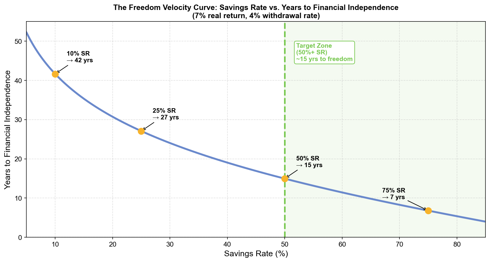
The inflection is visible around the 40–50% range: the slope steepens at lower savings rates and flattens at higher ones, but the shape makes the 50% region legible as the zone where the most leverage exists per additional percentage point saved.
What the Curve Means for Engineer Salaries
The Freedom Velocity Curve becomes most significant when viewed against actual tech salaries. A senior engineer in a major metro earning $200,000 total compensation with a 50% savings rate saves $100,000 per year. At 7% real return, this accumulates to the required 25× target in approximately 15 years.
The key insight is that the curve’s shape means small savings rate improvements early in your career have disproportionately large effects on the outcome. Consider three scenarios for a 30-year-old engineer earning $200,000:
Scenario A, 20% savings rate: $40,000/year. Annual expenses: $160,000. Portfolio target: $4,000,000. Time to FI: 33 years. Freedom at 63.
Scenario B, 30% savings rate: $60,000/year. Annual expenses: $140,000. Portfolio target: $3,500,000. Time to FI: 27 years. Freedom at 57.
Scenario C, 50% savings rate: $100,000/year. Annual expenses: $100,000. Portfolio target: $2,500,000. Time to FI: 15 years. Freedom at 45.
The difference between Scenario A and Scenario C is not doubling the savings. It is 2.5× the annual contribution while simultaneously reducing the target by 37.5%. The interaction between lower target and higher contribution rate is what produces the 18-year gap in freedom dates, not the savings amount alone.
The Curve as a Decision Framework
The Freedom Velocity Curve provides a direct answer to a common question: should I prioritize earning more or spending less?
At savings rates below 30%, spending reduction is the highest-ROI action because you are on the steep part of the curve. Each dollar of reduced spending does two things: it increases annual savings and decreases the FI target. Both effects together, on the steep slope, are worth more per dollar than any other financial intervention.
At savings rates above 50%, you are on the flat part of the curve. Further savings rate increases buy progressively fewer years. At this stage, income optimization (promotion, negotiation, career moves that increase earnings) becomes relatively more valuable, because the marginal time gain per additional saved dollar has diminished while the leverage of income on absolute portfolio size has not.
This implies a sequencing strategy:
- Get savings rate to 30% first (steep slope, high leverage per dollar of effort)
- Optimize income structure once savings rate is established
- Push toward 50% using income increases, not expense cuts (the target is already compressed by step 1)
- Beyond 50%, let compounding work; incremental tweaks matter less than time in market
The curve tells you not just where to go, but in what order to get there.
The Opportunity Cost of a Low Savings Rate
The Freedom Velocity Curve reframes the cost of lifestyle inflation in years, not dollars. A $10,000/year spending increase, upgrading from an adequate apartment to a premium one, moves you from, say, 30% savings rate to 25% savings rate on a $200,000 income. The curve says that shift costs approximately 4 additional years of mandatory employment.
Those 4 years are not hypothetical. They are years during which you will need to show up to work regardless of how the job is going, regardless of your manager, regardless of your health, and regardless of what else you would rather be doing. They are 4 years of optionality permanently traded for a better apartment.
The Freedom Velocity Curve makes that trade legible. It does not prohibit the trade. You may genuinely value the apartment more than the 4 years. But it requires you to make the trade consciously, with the correct price.
Most lifestyle upgrades are not declined after this analysis. But some are. And the ones that get declined are exactly the ones where the price in years turns out to exceed the value in satisfaction. The curve is the tool that surfaces those trades before they become permanent obligations.
The Crossover Line You Have Not Crossed Yet
The most common mistake engineers make on the Freedom Velocity Curve is starting an optimization sprint at a high savings rate (clipping subscriptions, refinancing, harvesting losses) while sitting at a 15% savings rate. The leverage on the curve at 15% comes from savings rate increases, not allocation optimization.
If you are below 30%, the curve is telling you one thing: increase the rate. The mechanism does not matter: higher income, lower expenses, or both. The metric that determines your position on the curve is the fraction, and the fraction is what the formula says governs the outcome.
The Crossover Point is 50%. Every percentage point of savings rate between your current number and 50% is on the steep part of the curve. Each one is buying back more years than the equivalent dollar amount at any other point in your financial life. The curve peaks at the beginning and fades as you approach the end. The time to be on the steep slope is now, not after you have already optimized everything else.
This article is adapted from Chapter 3 of Debugging Your Personal Finance, which presents the full Freedom Velocity Curve derivation and introduces the Crossover Point as the single most important threshold in the financial independence framework. Chapter 8 extends this into the Freedom Cross, the specific portfolio event where passive income overtakes active income requirements, and builds the monitoring system that tracks your approach to it in real time.
🧮Interactive tool: Savings Rate → Years to Financial IndependenceOpen →