There is a claim made in the FIRE (Financial Independence, Retire Early) community that engineers tend to resist because it violates intuition: your salary is irrelevant to how quickly you achieve financial independence. Not secondary. Not less important than savings rate. Literally irrelevant, mathematically eliminated from the formula.
This sounds wrong. More income means more savings, which means faster accumulation, which means earlier freedom. The chain of causation seems obvious. But the chain contains a hidden assumption: that income and expenses are independent variables. They are not. For most people, they are tightly coupled, and that coupling is what the algebra exposes.
This article derives the result from first principles. No approximations. No hand-waving. The derivation is four steps, each of which can be verified independently.
Step 1: The Financial Independence Condition
Financial independence has a precise definition: the moment your investment portfolio generates enough annual return to cover your living expenses without requiring additional labor income.
The safe withdrawal rate research, originally from William Bengen’s 1994 study and extended by the Trinity Study, establishes that a diversified equity portfolio can sustain a 4% annual withdrawal indefinitely across all historical market sequences, including the worst decades on record. This gives the FI condition:
Net Worth (NW) = Annual Expenses (E) / Withdrawal Rate (WR)At a 4% withdrawal rate, this simplifies to the Rule of 25: you need 25 times your annual expenses in invested assets to be financially independent. This is the target. This is the line you are trying to reach.
Step 2: The Accumulation Equation
Once you have a target, you need a model for how long it takes to reach it. Assume you save a fixed amount S each year and invest it at a real annual return r (inflation-adjusted). The future value of annual contributions compounding at rate r over t years is:
NW = S × [(1+r)^t − 1] / rThis is the standard future value of an annuity formula. It describes how your annual savings compound into a portfolio over time.
Setting Step 1 equal to Step 2, the target condition equal to the accumulation model:
E / WR = S × [(1+r)^t − 1] / rRearranging to isolate the ratio E/S:
E/S = WR × [(1+r)^t − 1] / rThis ratio E/S, expenses to savings, is what controls the timeline. The higher your expenses relative to savings, the longer the formula says you must work.
Step 3: The Cancellation
Now substitute the definitions of S and E in terms of income I and savings rate SR:
S = I × SR          (savings = income × savings rate)
E = I × (1 − SR)    (expenses = income × the part you don't save)
Calculate E/S:
E/S = [I × (1 − SR)] / [I × SR]
    = (1 − SR) / SR
The income I appears in both the numerator and denominator. It divides out completely. The ratio of expenses to savings depends only on the savings rate, not on the absolute value of income.
Substituting this back:
(1 − SR) / SR = WR × [(1+r)^t − 1] / rSolving for t:
(1+r)^t = [r × (1 − SR)] / [WR × SR] + 1

t = ln([r(1 − SR)] / [WR × SR] + 1) / ln(1 + r)
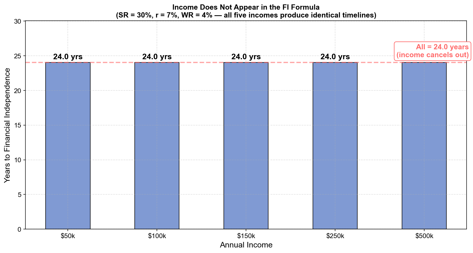
There is no I in this equation. Income has been algebraically eliminated. The time to financial independence is a function of three variables (savings rate, investment return, and withdrawal rate), and income is not among them.
Step 4: What the Formula Actually Says
The result has a specific interpretation. It does not say income is unimportant in absolute terms. It says that if you scale income and expenses proportionally, which is exactly what lifestyle creep does, the timeline does not change.
An engineer earning $80,000 who saves 30% ($24,000/year) and an engineer earning $400,000 who saves 30% ($120,000/year) will reach financial independence in exactly the same number of years. The second engineer will have a larger portfolio at the end, but the finish line, measured in years of work, arrives at the same time.
The chart makes the algebra visible.
Five income levels ($60k, $100k, $200k, $400k, $600k) are plotted against years to FI at savings rates from 10% to 60%. Every income level produces an identical curve. The lines are perfectly overlapping. The x-axis, savings rate, is the only variable that moves the result.
At 10% savings rate: approximately 42 years to FI, regardless of income. At 30% savings rate: approximately 27 years. At 50% savings rate: approximately 15 years. At 60% savings rate: approximately 12 years.
Income determines the size of the portfolio at freedom. Savings rate determines when freedom arrives.
The Hidden Assumption That Makes This Work
The formula has one critical assumption built in: that the savings rate is constant as a fraction of income. This is the assumption that lifestyle creep violates.
If a $200,000 engineer at 30% savings rate gets a $100,000 raise and increases spending to keep their savings rate at 30%, nothing changes; timeline unchanged. But if the same engineer keeps their savings in absolute dollars ($60,000/year) instead of as a fraction (30%), their expenses grow from $140,000 to $240,000/year, and their savings rate effectively drops from 30% to 20%. The formula says the timeline extends from 27 years to 37 years. A $100,000 raise, deployed incorrectly, costs 10 years of mandatory employment.
This is the “upskilling trap” the formula reveals. The raise feels like progress. The math shows it may be regression.
The counter-move is mechanical: when income increases, the savings rate (as a fraction, not as an absolute dollar amount) must also increase. If the raise adds $100,000 to annual income, the correct response is not to save the same $60,000 but to save 30% of the new $300,000, which is $90,000. The additional $30,000 redirected to savings versus lifestyle is the difference between timeline preservation and timeline extension.
The Non-Linearity of the Savings Rate
The formula is not linear. Improving your savings rate from 10% to 20% saves far more years than improving from 50% to 60%, even though both are 10 percentage-point increases.
| Savings Rate | Years to FI (7% return, 4% WR) |
|---|---|
| 10% | 42.5 years |
| 20% | 33.1 years |
| 30% | 26.8 years |
| 40% | 21.8 years |
| 50% | 15.4 years |
| 60% | 12.4 years |
| 70% | 8.7 years |
| 80% | 5.6 years |
The early savings rate improvements, getting from 10% to 30%, eliminate 15.7 years. The later improvements, 30% to 60%, eliminate another 14.4 years. The marginal return is highest when the rate is lowest, which means the most impactful intervention is almost always moving from low savings to moderate savings, not from moderate savings to aggressive savings.
The engineering implication: if you are saving less than 25%, the highest ROI action available to you is increasing the savings rate. Not optimizing asset allocation. Not negotiating a raise. Not tax-loss harvesting. Each of those is second-order compared to the first-order variable in the formula.
The Practical Derivation for Your Own Numbers
The formula requires three inputs: your savings rate SR, your expected real investment return r (7% is a commonly used historical average for a diversified equity portfolio), and your chosen withdrawal rate WR (4% is the standard conservative choice).
t = ln([r(1 − SR)] / [WR × SR] + 1) / ln(1 + r)At r = 0.07, WR = 0.04, SR = 0.30:
t = ln([0.07 × 0.70] / [0.04 × 0.30] + 1) / ln(1.07)
t = ln([0.049 / 0.012] + 1) / ln(1.07)
t = ln(4.083 + 1) / 0.0677
t = ln(5.083) / 0.0677
t = 1.626 / 0.0677 ≈ 24 years
The inputs are simple. The output is the number of years of working life remaining, not an estimate, not a range, but a precise mathematical consequence of the three variables you control.
You control savings rate directly. You influence investment return through asset allocation. You choose withdrawal rate based on risk tolerance. Income does not appear in any of those three levers. It was cancelled in Step 3. Acting as though it matters is optimizing for a variable that the formula already eliminated.
This article is adapted from Chapter 3 of Debugging Your Personal Finance, which derives this formula in full detail and extends it into the Freedom Velocity Curve, a visualization of how savings rate maps to years of working life across the full range of realistic scenarios. Chapter 8 introduces the Crossover Point: the specific portfolio level at which passive income overtakes active income requirements, ending the mandatory labor equation permanently.