The Engineering Proof of the 4% Rule: Lyapunov Stability for Retirement Withdrawals

The 4% rule is the most important constant in retirement planning, and almost nobody checks it the way an engineer checks a constant.

In engineering, we never ship a hard-coded number without asking what happens when the inputs move. This article runs that check on the 4% rule. It treats a retirement portfolio as a control system, writes down the equation that governs it, and then applies the tool control engineers use to certify walking robots and rocket engines, Lyapunov’s stability theorem, to a precise question: below what withdrawal rate does a retirement stay stable, and how much margin does a real retirement, with real markets and a finite length, need on top of that?

Written for two readers at once. If you enjoy the math, every step is here. If you do not, read the sentence after each equation, which says in words what it shows, look at the figures, and you will have the whole argument.

Where the 4% comes from

The rule of 25 says you can retire when your portfolio reaches 25 times your annual spending. If you spend 60,000 dollars a year, you need 1.5 million. The magic 25 is the inverse of a 4% safe withdrawal rate, since 1/0.04 = 25. The 4% itself comes from the work of William Bengen, who simulated 30-year retirements on historical market data. He searched for the SAFEMAX, the highest withdrawal rate that survived every historical retirement window, including the Great Depression, without the portfolio reaching zero. He found that a portfolio of 50% stocks and 50% bonds could sustain a 4.15% initial withdrawal rate, with the withdrawal raised each year for inflation.

As market conditions change, some researchers suggest a safer rate closer to 3%, while Bengen himself has more recently argued for 4.5% with small-cap value stocks. Later research extended his simulations with two variables the original study never had to handle, retirement horizon and starting valuation. A 30-year retirement and a 50-year one are different problems, and the failures cluster almost entirely in cohorts that retired into an expensive market. Starting from an expensive market, and over a horizon long enough to matter to anyone leaving work early, the safe rate drifts closer to 3.25% to 3.5% than to 4%. Christine Benz and her colleagues at Morningstar reach a similar place from a different direction, publishing an annual re-derivation of the safe rate from current bond yields and equity valuations. The 4% rule is best treated as the center of a distribution, and the question is what sets the shape of that distribution.

There is also a tempting shortcut. The S&P 500 has averaged roughly 10% a year, about 7% after inflation. If you withdraw 7%, shouldn’t you stay flat forever? You would not, because the market is neither linear nor predictable. The risk that breaks this intuition is sequence of returns risk, the risk of meeting negative returns early in your withdrawal phase. When the market drops in year one or two of retirement, you still have to sell shares to cover living expenses, locking in losses at the worst possible moment and permanently shrinking the base that future compounding works on. What matters is the order of returns as well as their average, and to see why, we need the dynamics of the portfolio.

Background for readers who are not engineers

Engineers describe anything that changes over time as a system. The system’s state is the number that describes it right now, here your wealth. The system’s dynamics are the rule for how that state changes from one moment to the next. A rule that links a quantity to its own rate of change is called a differential equation. The rate of change is written with a dot over the letter, so $\dot W$ (“W dot”) means “how many dollars per year your wealth is gaining or losing right now.” If $\dot W$ is positive, wealth is growing; if it is negative, wealth is shrinking.

An equilibrium is a state where nothing changes, so $\dot W = 0$. Stability is about what happens when something nudges the system away from equilibrium. Picture a ball. A ball at the bottom of a bowl is in a stable equilibrium: push it and it rolls back. A ball balanced on top of a hill is in an unstable equilibrium: the slightest push and it rolls away, faster and faster.

In 1892, the Russian mathematician Aleksandr Lyapunov found a way to prove which of the two you have without ever solving the equations of motion. His trick was to find one number that behaves like the system’s energy, always positive, and show that it can only go down. If such a number exists, the system has no choice but to settle, the way the ball’s altitude can only fall until it rests at the bottom of the bowl. That single idea is what we will apply to retirement.

Two more pieces of notation appear below. The number $e \approx 2.718$ is the base of continuous growth, so $e^{rt}$ means “something growing smoothly at rate $r$ for $t$ years.” The natural logarithm, $\ln$, undoes it, and it turns percentage changes into simple additions, which is why it shows up when returns are random. Here is every symbol in one place:

Symbol	Meaning
$W$	Your wealth, in today’s dollars
$W_n$	Your wealth in the dollars printed on your statement (nominal dollars)
$c$	What you withdraw per year, in today’s dollars
$r_{\text{nom}}$	The return on your statement (the nominal return)
$r_{\text{inf}}$	The inflation rate
$r$	The real return, $r_{\text{nom}} - r_{\text{inf}}$
$V$	Withdrawal stress, $c/W$, the share of remaining wealth withdrawn per year
$\sigma$	Volatility, the standard deviation of annual returns
$T$	The length of the retirement in years

Step 1: The equation that runs your retirement

Start with the dollars you actually see on your statement, your nominal wealth $W_n(t)$. At every instant, your account changes by what it earns minus what you take out. It earns the nominal return $r_{\text{nom}}$. The withdrawal is your lifestyle, $c$ a year at today’s prices, and to keep that lifestyle constant it has to rise with prices. If prices grow at the inflation rate $r_{\text{inf}}$, compounded once a year, the price level after $t$ years is $(1 + r_{\text{inf}})^t$ times today’s. Our equation describes change at every instant, so we compound in smaller steps instead. Splitting each year into $m$ steps that each raise prices by $r_{\text{inf}}/m$, and letting the number of steps grow to infinity, gives the price level of continuous compounding:

$$\begin{aligned} \text{Price level after } t \text{ years} &= \lim_{m \to \infty} \left(1 + \frac{r_{\text{inf}}}{m}\right)^{mt} \\ &= \left[\lim_{n \to \infty} \left(1 + \frac{1}{n}\right)^{n}\right]^{r_{\text{inf}} t} = e^{r_{\text{inf}} t} \end{aligned} \tag{1}$$

where we write the number of steps as $m = r_{\text{inf}}\,n$, and the limit inside the brackets is the definition of Euler’s number $e$. This equation shows that prices rising a little at every moment end up higher by a factor of $e^{r_{\text{inf}} t}$ after $t$ years, where $r_{\text{inf}}$ is the yearly inflation rate. At 3% inflation, prices after 10 years are 1.344 times today’s with yearly compounding and 1.350 times with continuous compounding, so the smooth version is a very close stand-in for the yearly one.

Multiplying today’s spending by this price level, the withdrawal in statement dollars is $c\,e^{r_{\text{inf}} t}$. Putting the return the account earns and this growing withdrawal together gives the rate at which your statement balance changes:

$$\dot W_n = r_{\text{nom}}\,W_n - c\,e^{r_{\text{inf}} t} \tag{2}$$

This equation shows that your statement balance grows by its return and shrinks by your withdrawal, where $\dot W_n$ is the change in the balance per year, $r_{\text{nom}}\,W_n$ is what the account earns, and $c\,e^{r_{\text{inf}} t}$ is the withdrawal, which keeps growing with prices. The return appears as a rate multiplying the balance, because the portfolio earns on whatever it holds at each instant. The withdrawal is an amount we choose, so we write it directly as a function of time. What your portfolio can buy at today’s prices is your wealth in today’s dollars, the statement balance divided by the price level:

$$W = W_n\,e^{-r_{\text{inf}} t} \tag{3}$$

This equation converts statement dollars into today’s dollars, where $W$ is your wealth in today’s dollars and $e^{-r_{\text{inf}} t}$ removes the price increase since you retired. Stability is about how wealth moves over time, so we need $\dot W$ written in terms of $W$ itself. Differentiating equation (3) with the product rule and substituting equation (2) for $\dot W_n$ gives

$$\begin{aligned} \dot W &= \dot W_n\,e^{-r_{\text{inf}} t} - r_{\text{inf}}\,W_n\,e^{-r_{\text{inf}} t} \\ &= \left(r_{\text{nom}}\,W_n - c\,e^{r_{\text{inf}} t}\right) e^{-r_{\text{inf}} t} - r_{\text{inf}}\,W_n\,e^{-r_{\text{inf}} t} \\ &= \underbrace{W_n\,e^{-r_{\text{inf}} t}}_{W}\;\underbrace{\left(r_{\text{nom}} - r_{\text{inf}}\right)}_{r} \;-\; c \end{aligned}$$

which leaves the equation that runs your retirement:

$$\dot W = r\,W - {c} \tag{4}$$

This equation shows that, measured in today’s dollars, your wealth grows by the real return and shrinks by your spending, where $r$ is the real return and $c$ is your yearly spending in today’s dollars. Inflation disappears from the equation because it hits both sides equally: it raises your withdrawal, and it eats the same share of your return. This does not make inflation harmless. Inflation cancels only because $r$ is already the real return, so the damage arrives through $r$ itself. Periods of high inflation, such as 1966 to 1982, have historically come with low real returns. The equation also rests on simplifying assumptions: the return and inflation are constant (we add randomness in Step 5), money grows and is withdrawn continuously, and there are no taxes or fees. Because the rates are continuously compounded, $r = r_{\text{nom}} - r_{\text{inf}}$ holds exactly. For rates compounded once a year, the exact relationship is $(1 + r) = (1 + r_{\text{nom}})/(1 + r_{\text{inf}})$, so a 7% nominal return with 3% inflation is a 3.88% real return, close to the 4% you get by subtracting. Your personal inflation can also run hotter than the consumer price index, and taxes are charged on nominal gains, so high inflation quietly raises the tax bill on returns that were never real gains.

Step 2: The equilibrium is a knife-edge

Now that we have the dynamic equation, we can find the portfolio’s equilibrium and test whether it is stable. Setting $\dot W = 0$ in equation (4) gives

$$W^{*} = \frac{c}{r} \tag{5}$$

This equation gives the one level of wealth at which nothing changes, where the star marks an equilibrium value: at $W^*$, the real return on your wealth exactly pays for your spending. With a real return of $r \approx 7\%$, the equilibrium sits at $W^* \approx 14.3c$. The rule of 25 ($W = 25c$) deliberately holds well above this line, and that margin is what makes it conservative.

To check stability, engineers nudge the system. Write your wealth as the equilibrium plus a small error, $W = W^* + \delta$. Substituting into equation (4) gives $\dot\delta = r\,\delta$, so $\delta(t) = \delta_0\,e^{rt}$. Because $r$ is positive, any error grows exponentially, so the equilibrium is unstable. A retiree who spends exactly what the portfolio earns is a ball balanced on a hilltop. One dollar below the target compounds toward bankruptcy, and one dollar above it compounds away into surplus, and the static rule of 25 gives no clue which way you will roll.

This small-nudge check tells us the direction of the danger, but not its size, and it says nothing about what happens far from equilibrium, when a retiree who started in 1966 takes a 40% drawdown in year three. For that we need Lyapunov.

Step 3: Lyapunov’s method and withdrawal stress

Lyapunov’s 1892 doctoral thesis, published in English translation in 1992, solved the long-standing problem of proving that a system is stable without solving its equations of motion. Classical methods could only prove stability for simple, idealized systems. Lyapunov’s move was to skip solving the dynamics entirely. His method asks you to find a positive scalar function, one that behaves like the system’s energy, and then to show that this energy never increases along any path the system can follow. If such a function exists, the system is provably stable. This is the same trick roboticists use to prove two-legged walking robots do not fall over, and the one aerospace engineers use to certify thrust-vector controllers that steer a rocket by rotating its engine nozzle.

For a retirement portfolio, the energy function I choose is the withdrawal stress, the annual withdrawal divided by the wealth that remains:

$$V = \frac{c}{W} \tag{6}$$

This equation defines stress as your current withdrawal rate, where $c$ is what you withdraw per year and $W$ is the wealth you have left. On day one of a 4% plan, stress is 4%. If your portfolio doubles, it falls to 2%, and if your portfolio halves, it jumps to 8%, so it measures how hard you are leaning on the portfolio right now. Stress is positive whenever wealth is finite. As wealth falls toward zero, stress explodes, and as wealth grows very large, stress fades toward zero, because a fixed withdrawal barely dents an enormous portfolio. Lyapunov’s method turns on whether stress rises or falls, so we differentiate it. Since $c$ is constant, the chain rule and equation (4) give

$$\dot V = -\frac{c\,\dot W}{W^2} = -\frac{c\,(rW - c)}{W^2} = \frac{c^2}{W^2} - r\,\frac{c}{W}$$

and replacing $c/W$ with $V$ turns this into a compact stability law:

$$\dot V = V\,(V - r) \tag{7}$$

This equation shows how fast stress changes, where $\dot V$ is the change in stress per year. It contains the entire engineering payoff, and it splits cleanly into two regimes. When $V < r$, the right side is negative, so stress decays and the portfolio grows faster than you withdraw from it. The retirement is stable, exactly the falling-altitude condition of the ball in the bowl. When $V > r$, the right side is positive, so stress compounds and every year you take out a larger fraction of a shrinking pile. The retirement is provably divergent and on a path to zero. The stability boundary sits exactly at

$$V_0 = {r} \tag{8}$$

This equation gives the largest initial withdrawal rate for which stress never rises, where $V_0$ is your withdrawal rate on the first day of retirement. If your withdrawal rate starts below your real return, it can only get smaller as the years go by. If it starts above, it can only get bigger, and it gets bigger faster and faster until the money is gone.

For engineers, the formal statement is that equation (7) has two equilibria, $V = 0$ and $V = r$. Taking $L(V) = V$ as the Lyapunov function, $\dot L = V(V - r) < 0$ for every $0 < V < r$, so $V = 0$ is asymptotically stable with region of attraction $[0, r)$, and $V = r$ is the unstable boundary of that region.

You can see both regimes in the figure below. The top panel plots the stability law itself, with the 4% rule sitting in the stable zone. The bottom panel follows stress over 50 years from different starting rates, with a constant 7% real return.

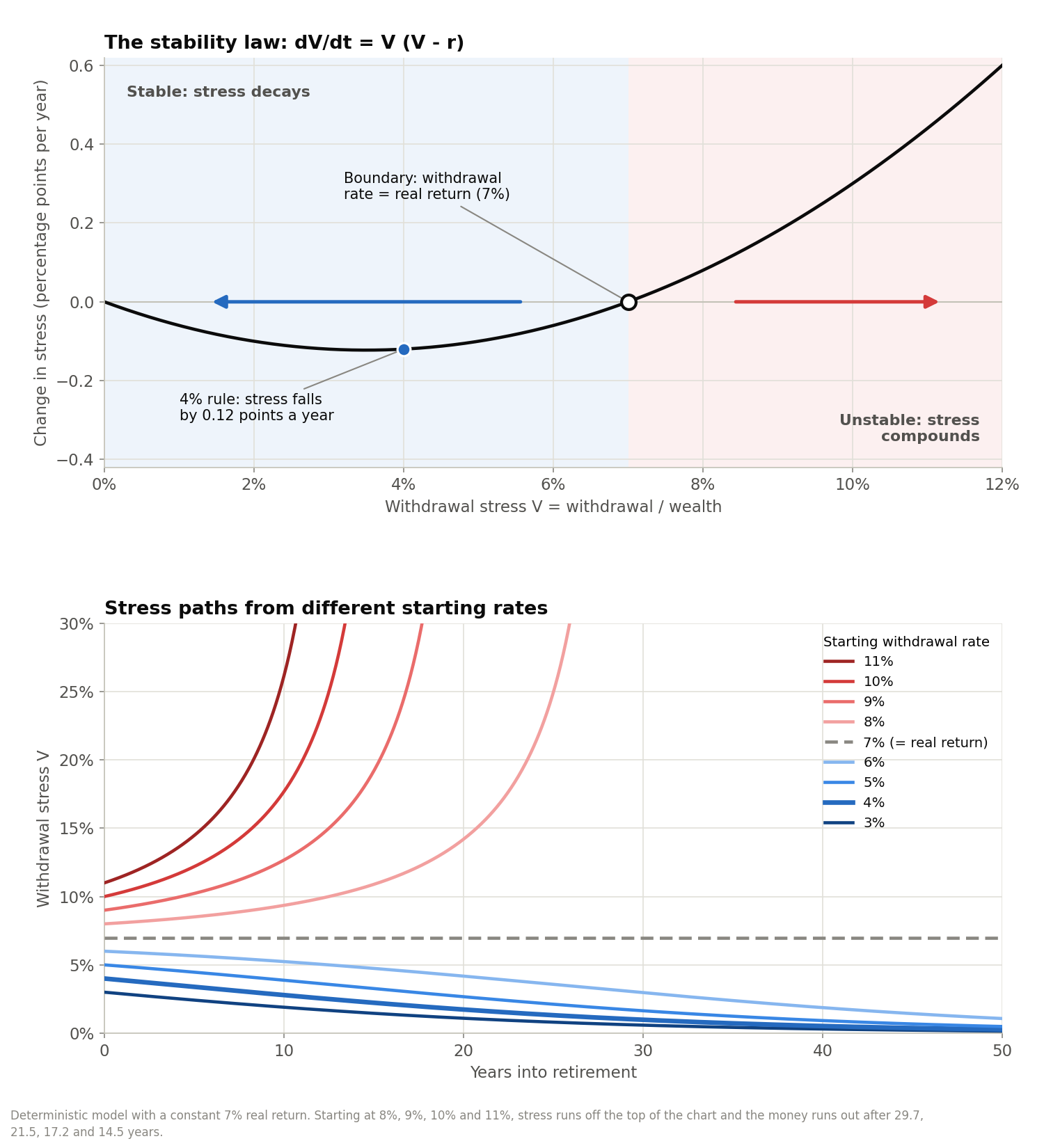
As you can see in the bottom panel, a retirement started at 8% with a 7% real return looks almost fine for a decade, then accelerates, and the money runs out after 29.7 years. Starting at 11%, it runs out after 14.5 years.

Step 4: Retirements end, so add time

The boundary $V_0 = r$ is a condition for an infinite horizon, which is a stronger promise than the one Bengen set out to test. His retiree only needs the money to last 30 years and is allowed to reach zero in the final month, so part of the principal can be spent along the way. We can bring time into the analysis by solving equation (4) for a retiree who starts with wealth $W_0$:

$$W(t) = \frac{c}{r} + \left(W_0 - \frac{c}{r}\right) e^{rt} \tag{9}$$

This equation shows your wealth after $t$ years, where $W_0$ is your wealth on the first day of retirement. Setting $W(T) = 0$, so the money runs out exactly at year $T$, gives the largest initial withdrawal rate that lasts $T$ years:

$$V_0^{\max}(T) = \frac{c}{W_0} = \frac{r}{1 - e^{-rT}} \tag{10}$$

This equation gives the largest withdrawal rate that lasts exactly $T$ years, where $T$ is the length of the retirement. With $r = 7\%$, a 30-year retirement allows about 8.0% and a 50-year one about 7.2%. As $T$ grows, $e^{-rT}$ shrinks toward zero and the rate falls back to $r$, the forever boundary of equation (8). A retirement with an end date can spend some principal, so it can start a little higher than the real return. The longer the retirement, the closer you have to stay to the forever boundary, which is why a 50-year early retirement needs a lower rate than Bengen’s 30-year one.

Step 5: Markets are random, so add volatility

So far the return has been perfectly steady. Real returns are stochastic, meaning they fluctuate randomly around their average, and the fluctuation itself costs money. A simple example shows why. Gain 50% one year and lose 50% the next, and your average return is zero, yet 100 dollars has become 150 and then 75. Losses hurt more than equal gains help. Over many years, wealth compounds at the average return minus half the variance of returns, a penalty that mathematicians call the geometric-mean correction and finance calls volatility drag.

The tool for doing calculus on randomly fluctuating quantities is Itô’s lemma, named after the Japanese mathematician Kiyoshi Itô who founded stochastic calculus. Give every instant’s return a random shock of size $\sigma$, so wealth follows $dW = (rW - c)\,dt + \sigma W\,dB_t$. Applying Itô’s lemma to the logarithm of stress gives

$$d(\ln V) = \left(V - r + \tfrac{1}{2}\sigma^2\right) dt \;-\; \sigma\,{dB_t} \tag{11}$$

This equation shows how the logarithm of stress moves when returns are random, where $\sigma$ is the volatility of the portfolio, the standard deviation of its annual returns, and $dB_t$ is a random shock with an average of zero, the unpredictable part of each instant’s return caused by news nobody could forecast. The oil price shock of 1973 and the COVID-19 crash of March 2020 are large negative shocks, a surprisingly strong earnings season is a positive one, and across many instants the good and bad surprises balance out on average.

The first term is the drift, the direction stress moves on average, and the second is the noise around it. The drift is negative, so stress falls on average, only while $V$ stays below a lower boundary:

$$V_0^{*} = r - \tfrac{1}{2}\sigma^2 \tag{12}$$

This equation gives the volatility-adjusted ceiling, where $V_0^{*}$ is the largest starting withdrawal rate whose stress still falls on average. Randomness moves the line: with bouncing returns, your stress falls on average only if your withdrawal rate stays below the real return minus half the variance of returns. With a 7% real return and 15% volatility, typical of US stocks, the line drops from 7% to 5.9%. A 50/50 stock and bond mix like Bengen’s loses less to volatility drag, but it also earns a lower return, and as we will see at the end of this article, the lower return wins and brings its ceiling close to his 4.15%.

To watch equation (12) at work, I simulated 20,000 retirements in an all-stock portfolio, built from the actual monthly real returns of the S&P 500 over the last 30 years. Over that period the average real return was 8.6% and the volatility 15.2%, which puts the ceiling at 7.4%. The figure below follows withdrawal stress in a retirement that starts at 4%, below the ceiling, and one that starts at 8%, above it.

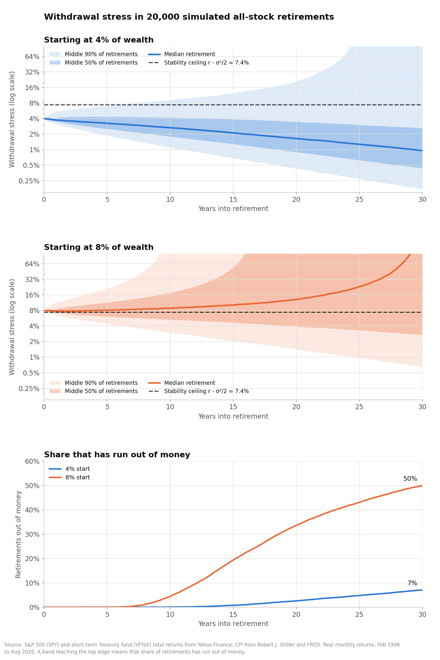
As you can see in the figure, the median retirement behaves exactly as equation (12) predicts. Started below the ceiling, its stress falls from 4% to about 1% over 30 years, meaning its real wealth roughly quadrupled. Started just above the ceiling, its stress drifts up slowly for a decade and then runs away. The bands show the other half of the story: around each median is a wide spread of luck, and that spread is what the next section is about.

What 20,000 simulated retirements say about time

There are two caveats we need to explore further. First, the drift in equation (11) describes what happens on average across many possible futures, but each retiree lives through only one of them. In that one future, the bad shocks can outnumber the good ones, for example when a crash arrives in the first years of retirement, and stress can rise even though the drift says it falls on average. A retiree below the boundary is stable on average but not guaranteed, so the longer the retirement, the more chances a bad run of returns has to push stress past the line.

To measure that effect, I simulated 20,000 retirements month by month for two portfolios, a 50/50 mix of the S&P 500 and short-term Treasuries and an all-stock portfolio. Each simulated retirement is built from 12-month stretches of the actual monthly real returns of the last 30 years, drawn at random, so it keeps the real streaks of good and bad months, such as 2000 to 2002 and 2008, that create sequence of returns risk. The simulation assumes the next 30 years look like a reshuffled version of the last 30, and for each retirement length it finds the largest withdrawal rate that still lasts in 95% of the simulated retirements. The figure below shows that rate next to the no-volatility rate from equation (10).

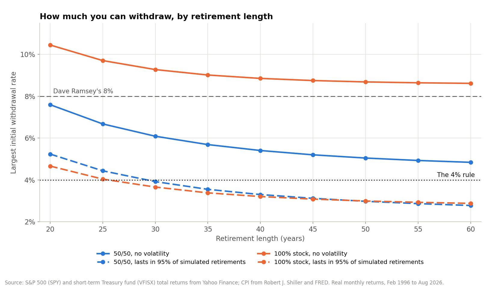
As you can see, for the 50/50 portfolio the rate that lasts in 95% of retirements is 3.9% over 30 years, a little below Bengen’s 4.15%, and it falls to 3.3% over 40 years and 3.0% over 50. The all-stock portfolio allows far more without volatility, 9.3% at 30 years, but once volatility and its real streaks are included it does no better than the 50/50 mix: 3.7% at 30 years and 3.0% at 50.

The gap between the two all-stock lines is so large because the volatility of stocks is twice that of the 50/50 mix, 15.2% against 7.7% a year, and the simulation charges for it twice. The figure below takes the 30-year rate apart, one cost at a time.

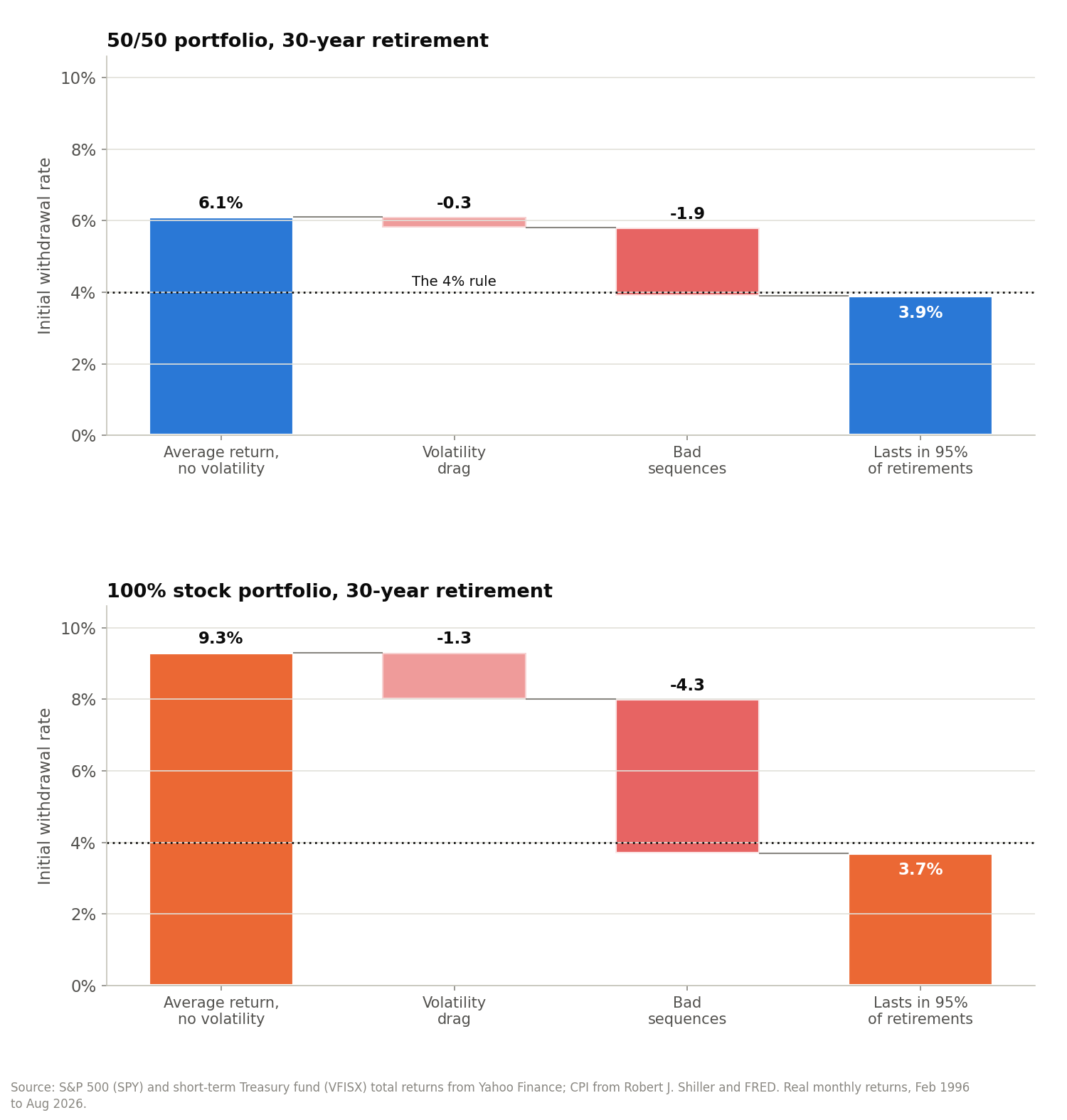
Volatility drag first lowers the growth rate of the portfolio in a typical retirement from the average real return of 8.6% to 7.4%, which brings the 30-year rate down to about 8%. Asking the money to last in 95% of retirements, and not just the typical one, then means surviving the retirements that draw the worst streaks early on, and that cuts the rate to 3.7%. For the 50/50 mix, the same two costs are much smaller, 0.3 and 1.9 points, because its volatility is half as large and the drag grows with the square of volatility.

Beyond about 50 years the order flips, and the all-stock rate edges above the 50/50 one, 2.9% against 2.8% at 60 years. Over a shorter retirement, the money runs out mainly because of a bad stretch in the early years, which the steadier 50/50 mix survives better. Over a very long one, the portfolio has to live on its growth for decades, and the higher return of stocks, compounding year after year, slowly outweighs the damage of their deeper crashes.

The average return tells you what a typical retirement can afford. A safe plan has to survive an unlucky retirement too, and for an all-stock portfolio, volatility and bad luck together cost more than half of what the average promised.

The 8% rule, tested

The gap between the two all-stock lines, with and without volatility, is not only of academic interest. In late 2023, the radio host Dave Ramsey argued on his show that an 8% withdrawal rate is fine, because good stock funds earn about 12%, inflation has averaged about 4%, and that “leaves you 8” (InvestmentNews, November 30, 2023). This is the intuition we discussed earlier, withdrawing the average real return, which is the forever boundary $V_0 = r$ of equation (8). For an all-stock portfolio, the no-volatility line in the figure above ends up at 8.6% as the retirement gets longer, close to Ramsey’s 8%. But that line assumes the average return arrives every single year. Once volatility is included, the all-stock rate that lasts in 95% of our simulated 30-year retirements is 3.7%, less than half of Ramsey’s 8%, and an 8% start ran out of money within 30 years in half of the simulated retirements. Nick Maggiulli’s historical analysis agrees with our stability analysis. He tested an 8% withdrawal from an all-stock fund over every 30-year retirement from 1935 to 2022, and the money ran out in 42% of them, mostly when the first decade brought poor real returns (Of Dollars And Data, November 14, 2023).

An 8% withdrawal sits above the stability ceiling of even an all-stock portfolio. It works when the early years are kind and fails roughly half the time when they are not, which makes it a coin flip on whether you run out of money.

Bengen asked a different question

The second caveat is that Bengen’s 4.15% answers a different question than ours. It is the largest rate that never ran out of money within 30 years in the historical record, including the 1966 cohort that retired into a recession, an oil shock, and a decade of double-digit inflation, and it allowed the withdrawal rate to rise along the way as long as the money lasted. A retiree who started in January 1973 with an all-stock portfolio and a 4% withdrawal saw the withdrawal rate stay above its starting value in every month of the next 30 years, peaking at 14.3%, and the money still lasted. Lyapunov’s condition is stricter, because it asks that the withdrawal rate never rise at all. That is what you need when the retirement has no end date, and for a retirement of a fixed 30 years it is more caution than Bengen’s test requires.

Can an equation prove anything about forever?

You may reasonably ask how an equation can prove anything about forever when $r$ and $\sigma$ are only averages of past data. It cannot, and it does not claim to. Lyapunov’s theorem proves something exact about the model: if your portfolio really earned a real return $r$ with volatility $\sigma$, a withdrawal rate below $r - \tfrac{1}{2}\sigma^2$ would see its stress fall on average for as long as you keep withdrawing. Whether the future delivers that $r$ is a separate question, and one that is very hard, almost impossible, to answer. Over the past century, stocks have risen over most long periods, but even the past comes with an error bar. An average of 30 annual returns, with a real average of 4.5% and a volatility of 7.7% for the 50/50 portfolio, pins the true mean down only to within about $7.7\%/\sqrt{30} \approx 1.4$ percentage points, one standard error either way.

So the proof tells you where the boundary sits for a given $r$, and the uncertainty in $r$ tells you how far below it to stay. Engineers handle every structure the same way, with an analysis that is exact for the design load and a safety factor that covers the fact that the real load is only estimated. The 4% rule is that safety factor, benchmarked against the worst sequence the US market has actually produced.

The ceiling across the stock and bond mix

Equation (12) also lets us run the sensitivity analysis across the entire allocation spectrum, because every portfolio mix trades expected return against volatility and therefore lands at a different ceiling. Using the same 30 years of real monthly data, with the S&P 500 as the equity engine and short-term Treasuries as the bond anchor, the figure below sweeps the blend from 100% bonds to 100% stocks. It shows the volatility-adjusted ceiling of equation (12) in blue and, for comparison, the simulated rate that lasts 30 years in 95% of retirements in green.

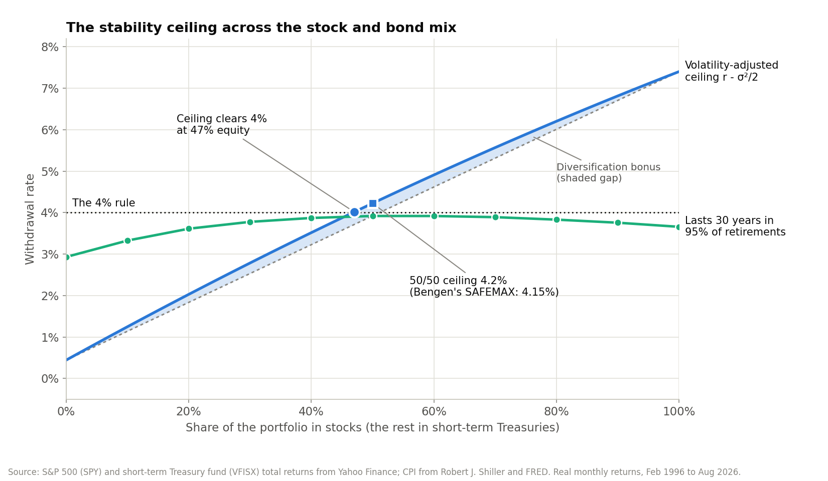
An all-bond portfolio earns so little in real terms that its ceiling sits near zero, far below 4%, meaning a bond-only retiree following the rule of 25 is unstable even in the model. The ceiling climbs steadily as stocks are added, clears the 4% line at roughly 47% stocks, and reaches about 7.4% for an all-stock portfolio, because over this period the extra return of stocks comfortably outpaced the volatility-drag penalty they carried. The 50/50 blend Bengen studied lands near 4.2%, strikingly close to his empirical 4.15% SAFEMAX. The two numbers answer different questions, but it is an encouraging sign that a one-line Lyapunov ceiling built from thirty years of data lands so near the answer his exhaustive historical simulation reached.

The curve looks almost straight at first glance, but the dotted reference line shows it is not. The blended return rises linearly with the share of stocks, while the volatility-drag penalty grows with the square of it, so the ceiling is a line minus a shallow parabola. The gentle upward bow above the straight-line blend, roughly a third of a percentage point at the 50/50 mix, is the diversification bonus: a mixed portfolio earns a higher ceiling than a simple average of the two ceilings it is built from.

The green line adds a result the ceiling alone cannot show. For a 30-year retirement, the rate that survives 95% of simulated retirements barely depends on the mix once stocks make up about a third of the portfolio, staying between 3.8% and 3.9% from 30% to 80% stocks and peaking at 3.9% around a 50/50 to 60/40 split. Even the all-bond portfolio sustains 2.9% for 30 years, far above its near-zero ceiling, because a retirement with an end date can spend its principal and a retirement that must last forever cannot. The forever ceiling keeps rewarding more stocks, while the 30-year rate flattens out, and the difference between the two is the difference between Lyapunov’s question and Bengen’s.

The 4% rule therefore quietly assumes a healthy share of stocks. Below about half in stocks, the portfolio cannot support 4% forever, while for a 30-year retirement, anything from roughly a third to four-fifths in stocks gives about the same safe rate, close to 3.9%.

What I take from the proof

The proof gives the 4% rule a mechanism. A withdrawal rate is stable when it sits below the real return minus half the variance of returns, and the 4% rule works because, for a balanced portfolio, it sits right at that line with the historical record as its safety factor. It also tells you where the rule stops working. For a 40- or 50-year early retirement, the simulation points to 3.0% to 3.3%. A portfolio with too few stocks has a ceiling below 4%. And a plan that withdraws the average return, like the 8% rule, sits above the ceiling of even an all-stock portfolio.

The most useful part, for me, is the variable itself. Withdrawal stress is a number you can compute every year from your own statement: this year’s spending divided by this year’s balance. A retiree whose stress is falling is in the stable regime, whatever the headlines say. A retiree whose stress has climbed toward the ceiling has an early warning, years before the balance looks alarming, and still has time to trim spending while the trim is small. That is how an engineer would run a retirement: with a stability margin designed in, and a feedback signal watched along the way.

This article is adapted from Chapter 4 of Debugging Your Personal Finance, which builds the rest of the system around this stability analysis: how to set the target, how to fund it, and how to keep it running.

How the numbers were made

The market data covers February 1996 to August 2026, 366 monthly returns. The S&P 500 is represented by the SPY fund and short-term Treasuries by Vanguard’s short-term Treasury fund (VFISX), both with dividends reinvested, from Yahoo Finance. Returns are converted to real terms with the consumer price index, from Robert J. Shiller’s dataset extended with FRED’s CPIAUCSL series. Portfolios are rebalanced monthly. Each simulated retirement is assembled from randomly drawn 12-month stretches of those real returns, 20,000 retirements per case, with a fixed random seed. Withdrawals are a constant real amount taken monthly, and a retirement fails in the first month its balance reaches zero. The largest rate that lasts in 95% of retirements is found by bisection. The “typical retirement” rate is the one that lasts in 50% of them.

Sources

• William P. Bengen, “Determining Withdrawal Rates Using Historical Data,” Journal of Financial Planning 7, no. 4 (1994): 171-180.
• William P. Bengen, “Choosing the Highest ‘Safe’ Withdrawal Rate at Retirement,” Financial Advisor Magazine (October 2020).
• Wade D. Pfau, “Safe Withdrawal Rates for Retirement,” Retirement Researcher (2018).
• Christine Benz, Jeffrey Ptak and John Rekenthaler, State of Retirement Income: How Retirees Can Determine a Safe Withdrawal Rate in 2025, Morningstar (2024).
• Michael Kitces, “Understanding Sequence of Return Risk & Safe Withdrawal Rates,” Kitces.com.
• Aleksandr M. Lyapunov, “The General Problem of the Stability of Motion,” International Journal of Control 55, no. 3 (1992): 531-773, English translation of the 1892 Kharkov doctoral dissertation.
• Kiyoshi Itô, “On Stochastic Differential Equations,” Memoirs of the American Mathematical Society 4 (1951): 1-51.
• Jeremy Siegel, Stocks for the Long Run, 6th ed. (McGraw Hill, 2022).
• Emile Hallez, “After Dave Ramsey Unleashes on 4% Rule, Advisors Unleash on Him,” InvestmentNews (November 30, 2023).
• Nick Maggiulli, “How Safe is an 8% Withdrawal Rate?” Of Dollars And Data (November 14, 2023).
• Market data: SPY and VFISX monthly total returns from Yahoo Finance; CPI from Robert J. Shiller’s online data (econ.yale.edu/~shiller) and FRED series CPIAUCSL.