There is a math error so common among high earners that it deserves its own name. Call it the Linearity Trap.
It works like this: an engineer in their mid-thirties decides to get serious about investing. They know they started late — maybe a decade behind where they should have been. Their internal model tells them the penalty is proportional. “I lost 10 years out of a 40-year runway. That’s 25% of the journey. I’m 25% behind. I’ll work a bit harder to close the gap.”
This model is wrong by a factor of two.
Starting 10 years late on a 40-year financial plan does not cost you 25% of your final wealth. It costs you closer to 50%. Sometimes more. The gap is not linear because the underlying system — compound interest — is not linear. And until you understand exactly why, you will continue applying linear-effort corrections to an exponential problem.
The Rule of 72 and the Geometry of Doubling
The fastest way to understand the cost of delay is not a spreadsheet. It is the Rule of 72.
At a 7% real annual return — the long-run historical average for US equities, derived from Jeremy Siegel’s analysis of 200 years of market data — money doubles approximately every 10.2 years (72 ÷ 7 = 10.3).
Now count the doubling periods available to you at different start ages, targeting retirement at 65:
| Start Age | Years Invested | Doubling Periods | Multiplier |
|---|---|---|---|
| 25 | 40 | ~3.9 ≈ 4 | 2⁴ = 16× |
| 35 | 30 | ~2.9 ≈ 3 | 2³ = 8× |
| 45 | 20 | ~1.9 ≈ 2 | 2² = 4× |
| 55 | 10 | ~0.97 ≈ 1 | 2¹ = 2× |
Look at the jump from age 35 to age 25. One decade of delay — losing a single doubling period — cuts the multiplier from 16× to 8×. That is exactly half. A dollar invested at 25 does not produce 25% more than a dollar invested at 35. It produces twice as much.
This is the math behind the Linearity Trap. The intuition says “10 years out of 40 = 25% loss.” The exponent says “one doubling period out of four = 50% loss.” These are not close. The engineer who delays by a decade is not a quarter behind. They are half behind, and no savings rate adjustment can fully compensate.
The Charlie and Cindy Simulation
Abstract percentages become concrete with a direct comparison.
Charlie starts investing at age 25. He puts $10,000 per year into a low-cost index fund for exactly 10 years — then stops completely. No further contributions. He simply lets the market compound. Total capital deployed: $100,000.
Cindy waits until age 35 — Charlie’s stopping point. Then she invests the same $10,000 per year, every single year, all the way to age 65. No stops, no pauses. Thirty years of disciplined, consistent contributions. Total capital deployed: $300,000.
Both target retirement at 65. Both earn the same 7% real return. At retirement:
| Investor | Capital Deployed | Years in Market | Final Value |
|---|---|---|---|
| Charlie | $100,000 | 40 years | ~$1.05M |
| Cindy | $300,000 | 30 years | ~$1.01M |
The chart below plots both trajectories to retirement.
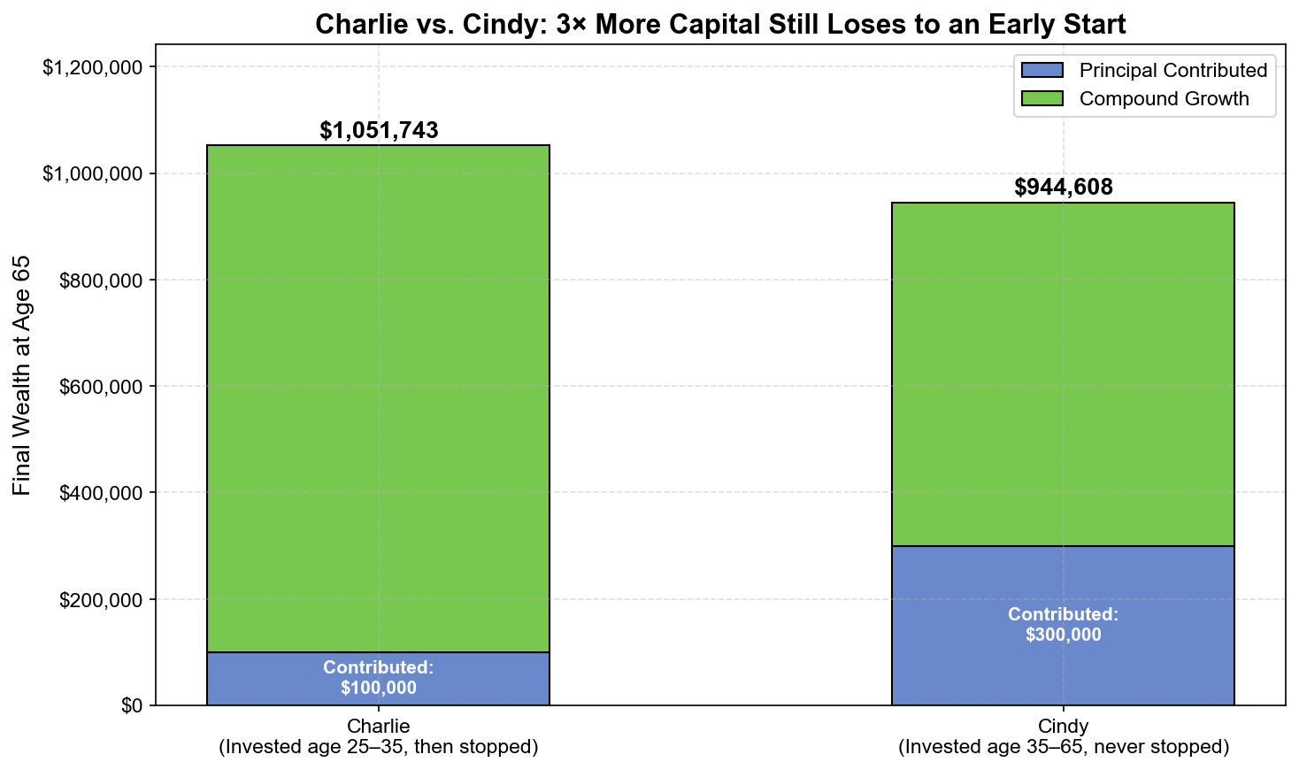
Cindy contributed three times more money than Charlie. She maintained perfect discipline for three decades while Charlie did nothing. She still lost.
The reason is not surprising once you understand doubling periods. Charlie’s early contributions each experienced four full doublings. Cindy’s contributions only experienced up to three. The extra doubling period — the most powerful one, when account balances are largest and each doubling produces the most absolute wealth — belonged exclusively to Charlie.
This is the compounding asymmetry that finance books mention in passing but rarely quantify directly: the first 10 years of investment are worth more than the next 20 years combined, because they determine how many doubling periods each dollar experiences. Cindy’s three decades of discipline could not buy back what Charlie earned in his first decade by simply starting early.
The Monthly Penalty Table
The Charlie-Cindy comparison shows the asymmetry in outcome. The monthly penalty table shows the cost in required effort.
Suppose your goal is to accumulate $1,000,000 by age 65, investing in an index fund returning 7% per year. How much do you need to set aside each month, depending on when you start?
| Start Age | Monthly Contribution | Total Contributed |
|---|---|---|
| 20 | ~$260/month | ~$140,400 |
| 25 | ~$380/month | ~$182,400 |
| 30 | ~$560/month | ~$201,600 |
| 35 | ~$820/month | ~$213,200 |
| 40 | ~$1,240/month | ~$223,200 |
| 45 | ~$1,940/month | ~$233,000 |
| 50 | ~$3,150/month | ~$252,000 |
The penalty ratio from age 20 to age 50 is 12.1×. The 50-year-old needs to invest $3,150 every month to achieve the same outcome the 20-year-old reaches with $260.
Read this table as a cost schedule. Every year you wait adds to the monthly payment required to reach the same destination — the same way interest accumulates on a debt you are not paying down. Except here, you are not paying interest to a bank. You are paying it to the math of compounding, and compounding collects on its own terms.
The other column worth studying is Total Contributed. The 20-year-old invests $140,400 total. The 50-year-old invests $252,000 total — nearly double — and still ends at the same finish line. More money out of pocket, more months of sacrifice, same result. The time advantage of the early starter is worth roughly $112,000 of principal that the late starter must make up through additional contributions.
What “I’ll Start When I Earn More” Actually Costs
This is the most common rationalization among high earners delaying financial action, and it contains a precise mathematical error.
“I’ll start when I earn more” treats the problem as being about P — the principal, the contribution amount. And it is true that P is under your control. Earn more, save more, contribute more. That is real and valuable.
But the future value formula is:
FV = P × (1 + r)^nP is a linear multiplier. Doubling P doubles your result. That is an O(n) optimization — useful, but expensive. n sits in the exponent. Losing one year of n reduces your final value by a factor that grows the longer you wait — an O(C^n) degradation.
“I’ll start when I earn more” is solving for the wrong variable. It is optimizing a linear input when the constraint is an exponential one. Every year of delay does not subtract a fixed amount from your final wealth. It removes an entire compounding layer — the same way removing the outermost term of a geometric series disproportionately shrinks the total.
There is no salary level that recovers a lost year of n. A 35-year-old who earns twice as much as their 25-year-old self but starts investing today has not undone the damage of a 10-year delay. They have increased P while permanently reducing n. The math does not allow a linear fix to an exponential problem.
The Only Irreversible Financial Decision
Most financial mistakes are recoverable. You can refinance a bad mortgage. You can rebuild an emergency fund. You can switch from bad mutual funds to low-cost index funds in an afternoon. These are setbacks, not catastrophes.
Time is the only truly irreversible variable. You cannot recover a lost doubling period. You cannot rewind a year of n. The compounding curve that was available to you at 25 does not exist at 35 — not at any savings rate, any income level, or any return assumption.
This is what the Linearity Trap costs: not just money, but irreversible optionality. Every month without capital deployed is a permanent reduction in the exponent. And the penalty compounds on itself, because each lost period is the one that would have multiplied everything that follows.
The practical implication is not complex. Start now, at whatever amount is available. If $50 per month is what is accessible, $50 is vastly better than waiting for the “right” amount. The 1-in-60 rule from the previous article tells you the heading matters more than the speed. The doubling period model tells you the same thing from a different angle: getting into the game early, even at low velocity, beats staying on the sideline at any velocity.
The most important financial decision you will make is not which fund to choose, which tax account to use, or how to optimize your allocation. It is the decision to deploy capital early — before the math becomes expensive.
The Correction Protocol for Late Starters
If you are reading this as a 35 or 40-year-old who has not started, the response is not despair. It is a recalibrated entry plan.
The standard rule of thumb — save 15% of income — was engineered for someone who started at 25 with all four doubling periods available. If you are starting a decade or more late, that rate simply stops the drift. It does not intercept the compound curve.
As covered in the aviation analogy, correcting a navigation error requires a double drift correction: an overcorrection angle that allows you to actually converge with the original flight path, not merely stop diverging. Applied to investing, that means a savings rate of 30% or more for late starters — aggressive enough to accelerate accumulation during the remaining doubling periods and partially offset the lost ones.
It will not be a perfect recovery. The arithmetic is honest about that. But the arithmetic also shows that the remaining doubling periods are still powerful. A 35-year-old with 30 years ahead still has three full doublings available. The 8× multiplier is still a multiplier. Starting now, with an aggressive correction, beats the alternative by a margin that compounds forward in your favor.
The question is never “can I fully recover the lost time?” You cannot. The question is “can I make the most of the time remaining?” You always can.
This article is adapted from Chapter 1 of Debugging Your Personal Finance, which builds the full mathematical case for early deployment and the engineering framework for staying on vector. Chapter 7 extends the latency analysis into real crisis simulations — bear markets, layoffs, and sequence-of-returns risk — showing exactly why time in the market outperforms timing the market across every historical window.