If you plug in a $1,000,000 stock portfolio with a $40,000 inflation-adjusted annual withdrawal into a smooth 7% spreadsheet, your balance will pass $3.8 million over thirty years. If you run the same portfolio through a bell-curve Monte Carlo simulator, the screen shows a reassuring 96.0% survival score.
Now, what if you force that retiree to start inside a three-year bear market built from the roughest one-year stretches in that historical record? Thirty-year survival drops to 55.8%. Almost half of those retirements run out of money, and the worst decile hits $0 at year 13.9.
The only difference between these two was how the simulator generated returns. Most spreadsheets and online calculators rely on statistical shortcuts that break up multi-year crash streaks before your money ever gets tested. You do not need to write software to see where they go wrong, because the math behind realistic market resampling comes down to one simple rule about time-series memory. Let’s see how it works under the hood in this article.
Why return order decides whether you run out of money
Over the past three decades, US stocks compounded at roughly 7.65% a year after inflation. Typing a flat 7.65% return into a retirement spreadsheet is a mathematical mistake. When you invest an untouched lump sum and never add or withdraw a dollar for months, ending wealth is a pure product of monthly growth factors:
where is your wealth after months, is the real (after-inflation) return in month , written as a decimal (0.02 for a 2% gain), and multiplies the growth factors of every month from to . Based on the above equation, the multiplication is commutative, so if you lose 30% in year one and gain 40% in year two, you end up with the exact same balance as gaining 40% first and losing 30% second.
Once you withdraw a constant real monthly living expense (~$3,333 a month, or $40,000 a year), portfolio wealth follows a path-dependent recursion instead:
If you unroll that recursion across just three months, you can get the idea why early returns carry far more weight than late returns:
Early return multiplies your entire starting capital , whereas late returns only compound whatever shares survived years of spending. Pulling $3,333 from a $1,000,000 portfolio liquidates 0.33% of your shares; pulling that inflation-adjusted $3,333 after a 50% drawdown liquidates twice as many shares at half the price, permanently shrinking the share base left to catch the eventual recovery. A smooth 7% projection sets that sequence penalty to zero by assumption.
From February 1996 through August 2026, we have 366 monthly inflation-adjusted total returns for US equities (SPY, tracking the S&P 500) and intermediate-term US Treasuries (VFITX, holding five-to-ten-year government bonds). Across those 30.5 years, $1.00 in SPY grew to $9.47 in constant purchasing power (7.65% real compound annual growth, 8.57% annualized arithmetic real mean, 15.26% volatility), while $1.00 in VFITX grew to $1.53 real (1.40% real compound rate, 5.08% volatility). Yet replaying that raw 1996-to-2026 timeline directly gives you a sample size of one where anyone retiring in February 1996 caught four booming dot-com boom years first, building a massive buffer before the 2000 crash arrived. Proper stress testing requires thousands of plausible alternate timelines without inventing fake market physics.
Why bell curves and single-month shuffles erase winter storms
Suppose you want to test whether your home’s plumbing can survive a Minnesota winter using 365 daily thermometer readings from last year. If you write all 365 daily temperatures on slips of paper, drop them into a hat, and draw 365 days one at a time with replacement, you will pull a -20°F January Tuesday sandwiched neatly between two 75°F July afternoons. Your pipes never freeze in the simulation because cold days were separated from winter. So standard retirement calculators have a similar error in one of two main ways:
- Bell-curve (Gaussian) Monte Carlo measures the historical monthly mean ( real for
SPY) and monthly standard deviation (), then draws 360 independent months from a normal distribution . That bell curve both understates extreme single months like October 2008 (-15.5% real in thirty days) and gives each month zero memory of the month before it. - Single-month shuffling (block length ) drops all 366 historical months into a hat and draws 360 isolated months with replacement. Every real crash month stays in the pool, yet drawing one month at a time scatters bear-market drops between calm summer gains just like shuffled thermometer slips.
For this, we can use block bootstrap resampling, and the figure below shows a step-by-step comparison of real clustered monthly returns and sliding 12-month blocks against a single-month shuffle that scatters crashes and a 12-month block bootstrap that stitches 30 intact blocks into a 30-year path.
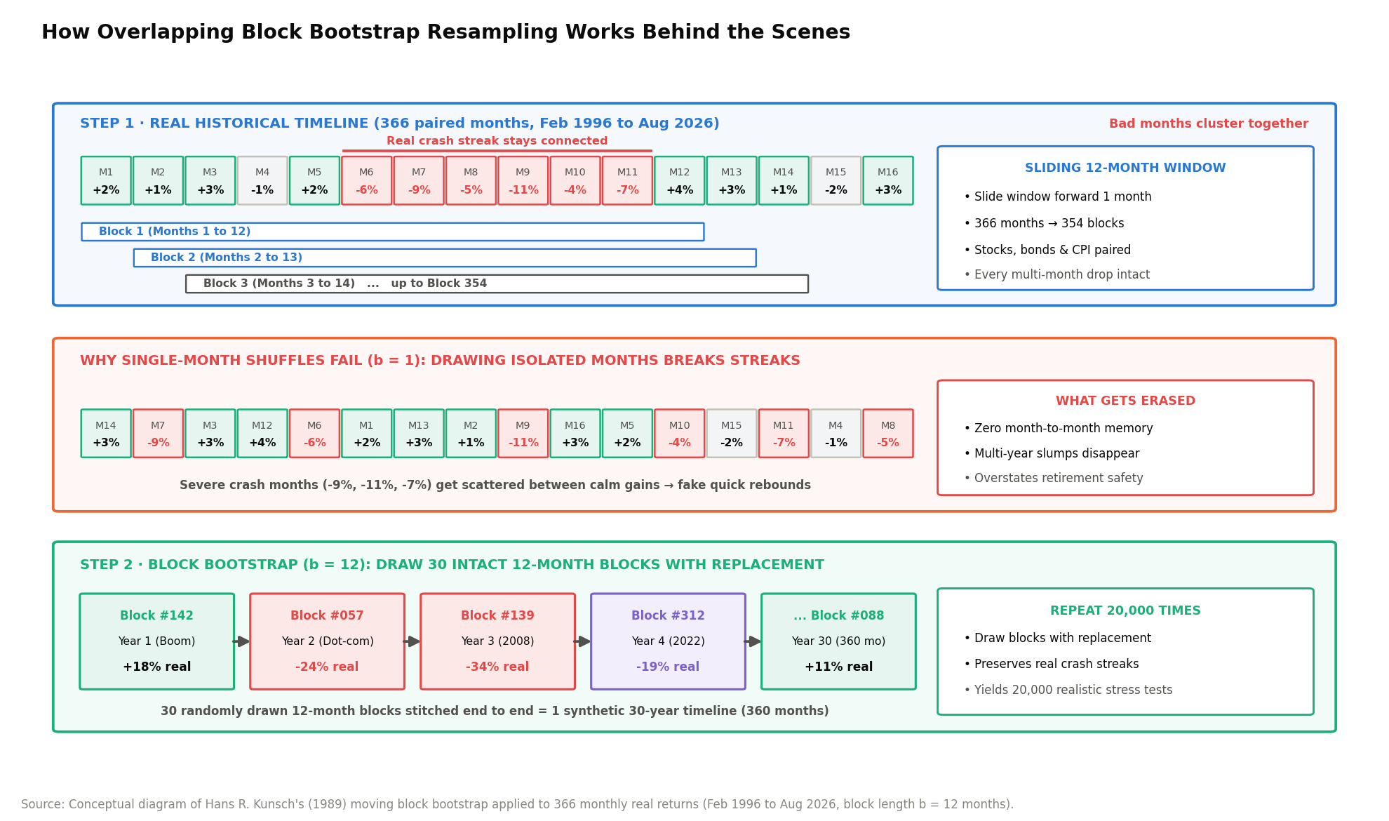
In the middle row above, severe crash months (-9%, -11%, -7%) get pulled in isolation, surrounded by positive months that create artificial instant rebounds.
Variance math explains why multi-year bear markets vanish under independent draws. Let denote the continuously compounded real return in month . Over an -month horizon (such as months, or three years), cumulative log return is , with variance:
where is the log return of month , is the number of months in the horizon, is the variance (the average squared distance of a value from its mean), and is the covariance between months and , positive when the two months tend to move in the same direction and negative when they move in opposite directions. The first sum adds up the risk of each month on its own, and the second adds the risk from every pair of months moving together. When months are drawn independently, every covariance is zero, and the variance of a three-year return is just the sum of its 36 monthly variances.
Even when month-to-month return direction shows weak linear predictability, market turbulence arrives in packs rather than isolated blips. A 10% monthly swing is far more likely to be followed by another violent swing than a quiet 1% gain, a property known as volatility clustering measured by the autocorrelation of absolute returns at lag :
where shows how strongly the size of this month’s move is tied to the size of the move months earlier, is the size of month ‘s return whether it was a gain or a loss, and is the correlation. Correlation is the covariance of two series divided by the product of their standard deviations, , which scales it to fall between -1 and +1. A value above zero, as in the equation, means a big move in one month makes another big move months later more likely, whether those moves are up or down.
Packing high-variance crash months into the same three-year window fattens cumulative loss tails far beyond what independent draws produce. When a simulator samples months independently, cross-month memory collapses to zero, and summing 36 independent draws washes out sustained bear markets via the central limit theorem. Below, I ran 20,000 simulated 30-year S&P 500 timelines (random seed 2026) across matched Gaussian Monte Carlo, a single-month shuffle (), and an overlapping 12-month block bootstrap ().
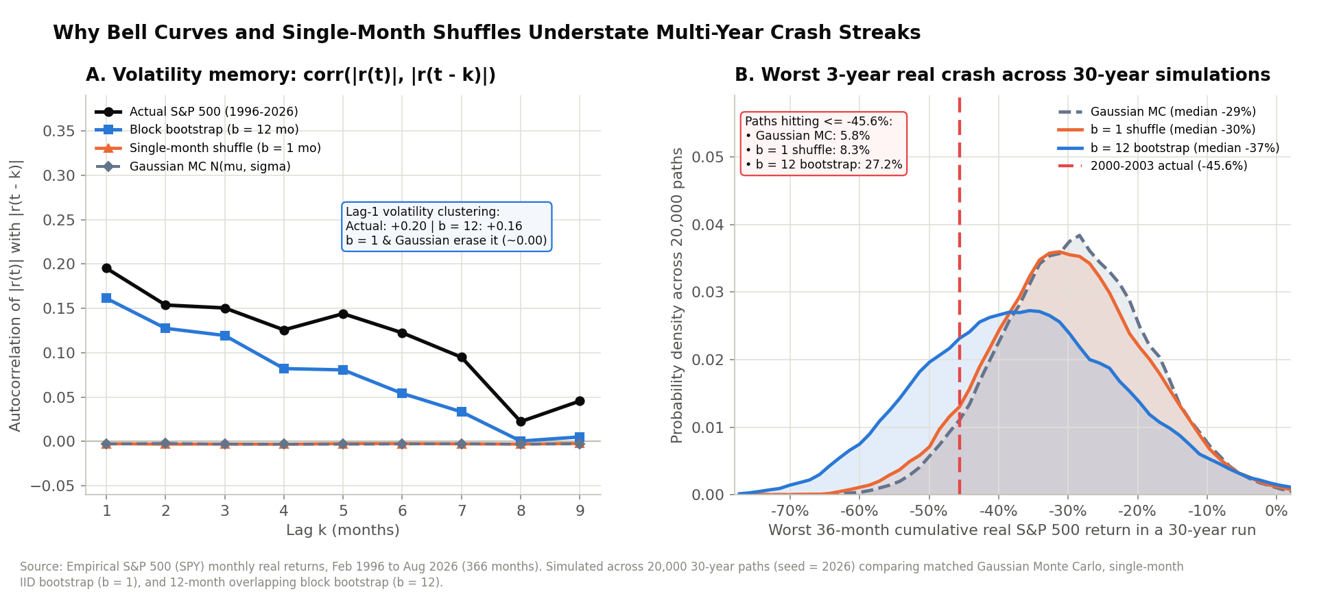
Panel A tracks turbulence memory across lags to months. In actual 1996-2026 SPY data, lag-1 volatility clustering sits at +0.20 (+0.195), lag 2 sits at +0.15, and positive clustering persists out to seven months. Under both Gaussian draws and single-month shuffling, drops flat to 0.00 (-0.003) at every lag: draw October 2008 in month fourteen of a single-month shuffle, and month fifteen has no idea credit markets are frozen.
Panel B shows what erasing that memory does to three-year bear markets. Between April 2000 and March 2003, the S&P 500 lost 45.6% of its real purchasing power over 36 months. Across 20,000 simulated 30-year lifetimes, how often does each engine suffer a 36-month cumulative real return of -45.6% or worse?
- Gaussian Monte Carlo produces a -29.0% median worst 36-month slump (10th percentile -42.5%), reaching -45.6% or worse in just 5.8% of lifetimes.
- Single-month shuffling () nudges the median worst slump to -30.3% (10th percentile -44.4%), reaching -45.6% or worse in only 8.3% of lifetimes.
- Overlapping 12-month block bootstrap () deepens the median worst slump to -36.7% (10th percentile -54.7%) and hits -45.6% or worse in 27.2% of lifetimes, 4.7 times as often as a bell curve and 3.3 times as often as a single-month shuffle.
The math behind block bootstrap
Statistician Hans R. Künsch introduced the moving block bootstrap in The Annals of Statistics (1989) to resample time series without severing short-range serial dependence. Rather than drawing individual observations, you slice the historical record into overlapping contiguous strips of length and sample intact strips with replacement.
Start by converting each asset’s nominal monthly total return into real terms using that calendar month’s Consumer Price Index inflation rate :
where is the real (after-inflation) return in month , is the nominal return before inflation, and is that month’s inflation rate, the change in the Consumer Price Index (CPI), which tracks the prices of a basket of goods and services that households buy. At monthly CPI rates near 0.2%, linear subtraction matches exact Fisher division within a few hundredths of a percent and is used directly in our simulation, embedding real inflation spikes inside every return rather than assuming a tame 2.5% inflation rate. Next, lock all assets from calendar month into a paired return vector:
Across monthly observations with block length , while twelve-month windows fit inclusive of the final boundary month, indexing start dates across the first months forms the pool of 354 overlapping 12-month blocks used in our simulations:
Sliding the window forward one month at a time beats slicing neat January-to-December calendar years for two reasons. Calendar slicing would leave only 30 non-overlapping blocks across three decades instead of 354 distinct entry points, and real market crises ignore New Year’s Day where during the Global Financial Crisis from November 2007 through February 2009, SPY fell 51.5% in real terms while VFITX gained 12.1%.
Pairing stocks and bonds inside the same monthly vector also preserves regime-dependent cross-asset behavior without imposing a static correlation matrix. During the dot-com bust from September 2000 to September 2002, SPY dropped 47.3% in real terms while VFITX rallied 24.3%. During 2022, an inflation shock hit SPY (-23.3% real) and VFITX (-16.0% real) simultaneously, flipping real monthly stock-bond correlation from -0.19 (1996-2021) to +0.54 (2022-2026). Whenever a simulated path draws a 2008 window, Treasuries cushion equities; whenever it draws a 2022 window, both assets fall together just as they did in real life.
To build one synthetic 30-year (360-month) future, draw block start indices independently and uniformly with replacement, assigning each block probability , and concatenate those thirty strips end to end:
Sampling with replacement puts every 12-month strip right back into the pool after each draw, allowing an unlucky path to pull two 2001 blocks and a 2008 block in its opening five years while a calmer path draws mostly expansions. Stitching 30 draws from 354 blocks yields distinct 30-year sequences while keeping 11 of every 12 consecutive monthly transitions (91.7%) completely intact.
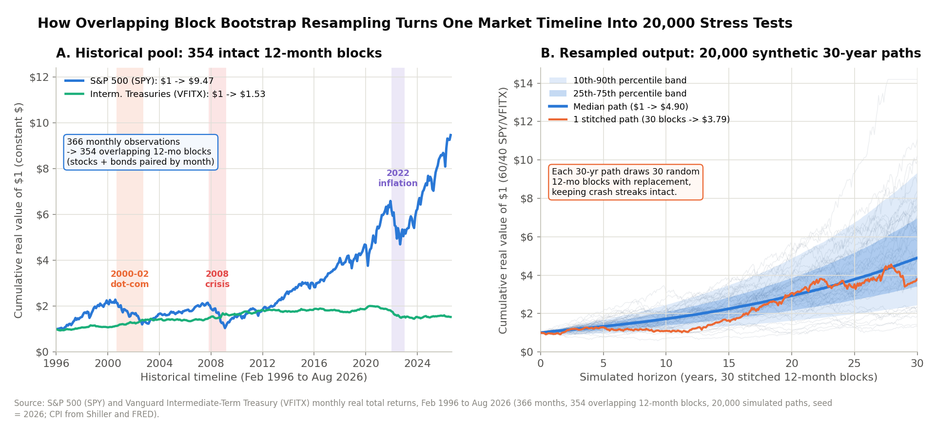
The figure below shows these steps on real data. Panel A is the pool we draw from, the after-inflation growth of $1 in SPY and $1 in VFITX from February 1996 to August 2026, with the dot-com bust, the 2008 crisis, and the 2022 inflation shock shaded. We cut this one timeline into 354 overlapping 12-month blocks, keeping stocks and bonds from the same month together. In Panel B each faint gray line is one 30-year path stitched from 30 randomly drawn blocks, the orange line follows a single path from start to end, the thick blue line is the median path, and the shaded bands hold the middle 50% and 80% of all 20,000 paths.
Without going deep on how it works with coding, the entire simulation can be explained in five steps:
- Subtract each month’s CPI inflation rate from that month’s stock and bond total returns across all 366 historical months, keeping stock and bond returns from the same calendar month locked on the same row.
- Form overlapping 12-month strips by grouping Rows 1 to 12 as Block 1, Rows 2 to 13 as Block 2, Rows 3 to 14 as Block 3, and continuing through Block 354.
- Draw 30 strips at random with replacement, returning each strip to the pool after every pick, and stack those thirty 12-month strips end to end into one 360-month timeline.
- Step your portfolio forward month by month along that timeline and apply that row’s real returns, subtract your constant-dollar monthly withdrawal, rebalance according to your target weights, and flag whether the balance ever touches $0.
- Repeat Steps 3 and 4 twenty thousand times and rank all 20,000 outcomes from worst to best to read off survival probability, median ending wealth, and the 10th-percentile worst-decile trajectory.
Before turning withdrawals back on, Panel B in the figure above shows pure compounding across 20,000 stitched paths for a $1.00 lump sum in a monthly rebalanced 60/40 SPY/VFITX mix where median 30-year purchasing power reaches $4.90, spanning $2.44 at the 10th percentile to $9.34 at the 90th, while retaining +0.16 lag-1 volatility clustering compared to +0.20 in raw history.
Choosing the block length and testing a bad start
Now let’s go back to the introduction of this article and see how we get to those numbers. We should see how sensitive a $1,000,000 portfolio withdrawing $40,000 a year in constant dollars ($3,333.33 per month, the 4% rule) is to the block length . The chart below tests matched bivariate Gaussian Monte Carlo alongside block lengths of 1, 3, 6, 12, 24, 36, and 60 months across 20,000 retirements per engine.
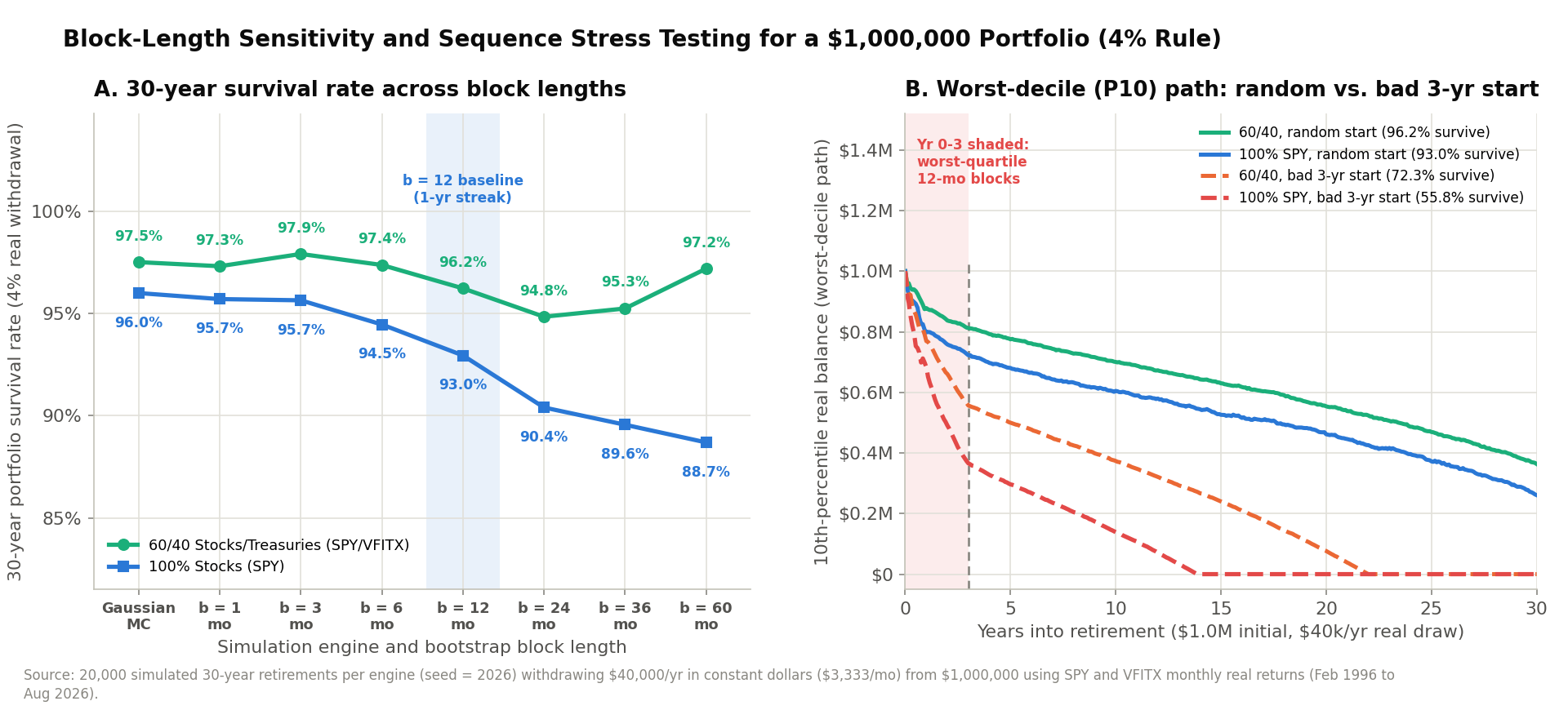
In Panel A of the figure above, an all-equity (100% SPY) retirement prints a 96.0% survival rate under Gaussian draws and 95.7% under a single-month shuffle (). Keeping intact 12-month strips together () lowers survival to 93.0%, nearly doubling the failure rate from 4.0% to 7.0%, and longer blocks trim survival further to 90.4% at and 88.7% at . Pairing 60% equities with 40% intermediate Treasuries (SPY/VFITX) holds survival remarkably steady across every engine: 97.5% under Gaussian draws, 96.2% at , 94.9% at , and 97.2% at .
Selecting months as the baseline balances a finite-sample bias-variance trade-off documented by Philippe Cogneau and Valeri Zakamouline (Quantitative Finance, 2013):
- Very short blocks (1 or 3 months) sever intra-year volatility clustering and bear-market momentum, understating multi-year drawdowns.
- Very long blocks (36 or 60 months) leave barely six non-overlapping five-year windows inside a 30.5-year sample, recycling the exact multi-year recoveries of one historical era.
- Twelve-month blocks keep full four-quarter bear-market legs and inflation shocks intact across 354 distinct windows. Because splicing independent one-year strips cuts across decade-long mean-reversion cycles (where deep multi-year bear markets historically preceded stronger ten-year recoveries), Cogneau and Zakamouline showed that moving block bootstraps near slightly widen 30-year equity dispersion, erring on the side of caution rather than false safety.
Block resampling also makes conditional bad-start stress testing straightforward (Panel B above). Rank all 354 twelve-month SPY strips from worst to best and isolate the bottom quartile where 89 strips return +1.9% real or less, averaging -13.9% real per year. Forcing Years 1 through 3 of retirement to sample exclusively from those 89 rough strips before letting Years 4 through 30 draw freely from all 354 blocks exposes pure sequence-of-returns fragility:
- All-equity (100%
SPY) 30-year survival drops from 93.0% to 55.8%, and the 10th-percentile path runs out of money at year 13.9. - Balanced 60/40 (
SPY/VFITX) survival holds at 72.3%, 16.5 percentage points higher, extending worst-decile solvency by 8.1 years out to year 22.0.
Eight additional years of the worst-decile runway buys nearly a decade to trim discretionary spending by 10% or draw from a dedicated cash buffer instead of selling depressed shares at the bottom. When you test your own retirement numbers in the Portfolio Simulator or Early Retirement Calculator, look past unconditional 95% averages and check how your allocation holds up when three rough years arrive right out of the gate.
Adapted from the block bootstrap simulation framework in Chapters 3 and 4 of Debugging Your Personal Finance.
Sources
- Künsch, Hans R. (1989). “The Jackknife and the Bootstrap for General Stationary Observations.” The Annals of Statistics, 17(3), 1217-1241.
- Cogneau, Philippe, and Valeri Zakamouline (2013). “Block Bootstrap Methods and the Choice of Stocks for the Long Run.” Quantitative Finance, 13(9), 1443-1457.
- Yahoo Finance monthly total returns (
SPY,VFITX) deflated with Robert J. Shiller CPI and FREDCPIAUCSL, Feb 1996 to Aug 2026 (366 months, 354 overlapping 12-month blocks, 20,000 simulated paths, random seed 2026).